Environmental Geophysics
Induced Polarization
Introduction
Conrad Schlumberger (Dobrin 1960) probably was first to report the induced polarization phenomenon, which he called "provoked polarization." While making conventional resistivity measurements, he noted that the potential difference, measured between the potential electrodes, often did not drop instantaneously to zero when the current was turned off. Instead, the potential difference dropped sharply at first, then gradually decayed to zero after a given interval of time. Certain layers in the ground can become electrically polarized, forming a battery when energized with an electric current. Upon turning off the polarizing current, the ground gradually discharges and returns to equilibrium.
The study of the decaying potential difference as a function of time is now known as the study of induced polarization (IP) in the time domain (figure 1a). In this method the geophysicist looks for portions of the earth where current flow is maintained for a short time after the applied current is terminated. Another technique is to study the effect of alternating currents on the measured value of resistivity, which is called IP in the "frequency domain" (figure 1b). In this method the geophysicist tries to locate portions of the earth where resistivity decreases as the frequency of applied current is increased. The induced electrical polarization method is widely used in exploration for ore bodies, principally of disseminated sulfides. Use of IP in geotechnical and engineering applications has been limited, and has been used mainly for groundwater exploration. Groundwater IP studies generally have been made with time-domain IP.
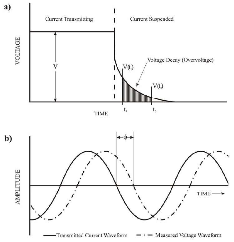
Figure 1. (a)Time domain and (b)frequency domain waveform illustrations (Glaser, 2007).
General Theory of the IP Effect
The origin of induced electrical polarization is complex and is not well understood. This is primarily because several physio-chemical phenomena and conditions are likely responsible for its occurrence. Only a fairly simple discussion will be given here. According to Seigel (1970), when a metal electrode is immersed in a solution of ions of a certain concentration and valence, a potential difference is established between the metal and the solution sides of the interface. This difference in potential is an explicit function of the ion concentration, valence, etc. When an external voltage is applied across the interface, a current is caused to flow, and the potential drop across the interface changes from its initial value. The change in interface voltage is called the "overvoltage" or "polarization" potential of the electrode. Overvoltages are due to an accumulation of ions on the electrolyte side of the interface waiting to be disged. The time constant of buildup and decay is typically several tenths of a second.
Overvoltage is therefore established whenever current is caused to flow across an interface between ionic and electronic conduction. In normal rocks, the current that flows under the action of an applied emf does so by ionic conduction in the electrolyte in the pores of the rock. There are, however, certain minerals that have a measure of electronic conduction (almost all the metallic sulfides (except sphalerite) such as pyrite, graphite, some coals, magnetite, pyrolusite, native metals, some arsenides, and other minerals with a metallic lustre). Figure 2 is a simplified representation of how overvoltages are formed on an electronic conducting particle in an electrolyte under the influence of current flow.
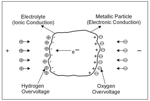
Figure 2. Overvoltage on a metallic particle in electrolyte. (Seigel 1970; copyright permission granted by Geological Survey of Canada)
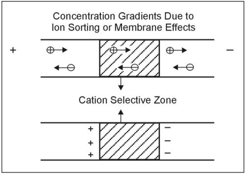
Figure 3. Nonmetallic induced polarization agent. (Seigel 1970; copyright permission granted by Geological Survey of Canada)
The most important sources of nonmetallic IP in rocks are certain types of clay minerals (Vacquier 1957, Seigel 1970). These effects are believed to be related to electrodialysis of the clay particles. This is only one type of phenomenon that can cause "ion-sorting" or "membrane effects." For example, figure 3 shows a cation-selective membrane zone in which the mobility of the cation is increased relative to that of the anion, causing ionic concentration gradients and therefore polarization. A second group of phenomena includes electrokinetic effects that produce voltage gradients through the `streaming potential' phenomenon. These voltage gradients will have the same external appearance as polarization effects due to separation of ge. Electrokinetic effects seem less important than membrane effects in the overall polarization picture.
In time-domain IP, several indices have been used to define the polarizability of the medium. Seigel (1959) defined "chargeability" (in seconds) as the ratio of the area under the decay curve (in millivolt-seconds, mV‑s) to the potential difference (in mV) measured before switching the current off. Komarov, et al., (1966) defined "polarizability" as the ratio of the potential difference after a given time from switching the current off to the potential difference before switching the current off. Polarizability is expressed as a percentage.
Seigel (1959) showed that over a heterogeneous medium comprised of n different materials, apparent chargeability ηa is approximately related to apparent resistivity by
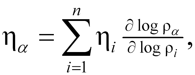 (1)
(1)
where
ηi = chargeability of the ith material,
ρi = resistivity of the ith material.
Seigel provided the validity of
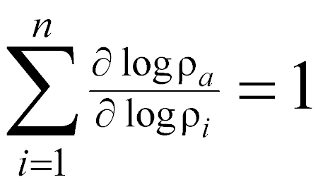 (2)
(2)
Equations 1 and 2 yield the useful formula for ha/h1:
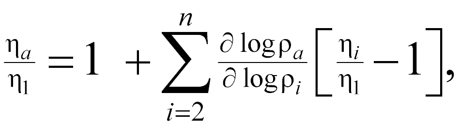 (3)
(3)
If the theoretical expression for apparent resistivity ρa is known, then the corresponding expression for the reduced apparent chargeability ηa/ηi can be derived.
Spectral Induced Polarization
Spectral Induced Polarization (SIP) measures the variation of resistivity with frequency. The method, therefore, requires several resistivity measurements at different frequencies. These can be recorded in the frequency domain or in the time domain. In the time domain, where voltage measurements are recorded after the transmitting current has been turned off, the decaying voltage is sampled several times as it decays. Using the Fourier Transform, these data can be transformed into the frequency domain providing resistivity values at different frequencies.
SIP measurements are occasionally used in mineral exploration to assist in identifying graphite and clay from sulfide mineralization. In addition, some information about the habit of the polarizable minerals could be obtained. It can also be used to map clay and, in some cases, contamination.
Sounding and Profiling
The techniques of sounding and profiling, used in resistivity measurements, are also used in the IP method. IP soundings are most commonly made using the Schlumberger array, pole-dipole array, or Wenner array, and usually in the time domain. The apparent chargeability ηa versus the electrode spacing a is plotted on logarithmic coordinates. The IP sounding curve is an interpreted curve matching procedures, either graphically, using sets of IP sounding master curves, or by computer. At present, only a few two-layer master curves (for the Wenner array) have been published in the United States (Seigel, 1959; Frische and von Buttlar, 1957). Three- and four-layer curves have been published in the Soviet Union.
An IP sounding curve can be of significant value in complementing a resistivity sounding curve. For example, the resistivity and IP sounding curves for the following four-layer geoelectric section are shown in figure 4:
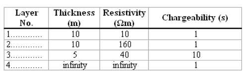
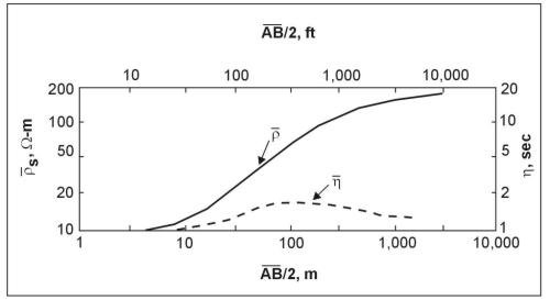
Figure 4. Apparent resistivity and apparent chargeability (IP) sounding curves for a four-layer model. (Zohdy 1974a, 1974b)
It is obvious that layer 3 cannot be distinguished on the four-layer resistivity curve (which resembles a two- or three-layer curve). But layer 3 is characterized by a different chargeability from the surrounding layers, and its presence is indicated clearly by the IP sounding curve.
When profiling, the pole-dipole or dipole-dipole (see figure 5) arrays are used almost exclusively. It can be easily employed in the field using short lengths of wire or multi-conductor cables allowing several values of the spacing multiplier (n) to be measured from one current dipole location. For one or two values of n, the IP and resistivity results are plotted as profiles. For more than two values of n, the profile method of presentation becomes confusing. A two-dimensional (usually called pseudosection) format has been developed to present the data (figure 5). This form of presentation helps the interpreter separate the effects of IP and resistivity variations along the line from vertical variations. The 45° angle used to plot the data is entirely arbitrary. The pseudosection plots are contoured, and the resulting anomalous patterns can be recognized as being caused by a particular source geometry and/or correlated from line to line. However, the contoured data are not meant to represent sections of the electrical parameters of the subsurface (Hallof, 1980). The pseudosection data plots are merely a convenient method for showing all of the data along one given line in one presentation.
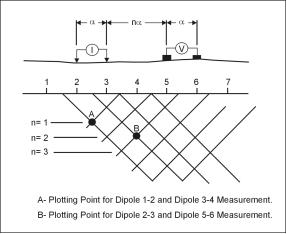
Figure 5. Dipole-dipole plotting method.
Cross Borehole Imaging
Cross borehole imaging, or tomography, employs similar techniques as those used in soundings and profiling, resulting in an electrical cross section of the resistivity or IP property distribution. The technique has been used for many different applications including: permeable reactive barrier (PRB) integrity imaging, hydrocarbon contaminant mapping, groundwater infiltration timeseries imaging, tracer studies, permeability and transmissivity estimation, etc. Figure 6 presents an example of resistivity and IP tomography data taken from a hydrocarbon contaminated (kerosene) site. The soil column shows a fine grained layer at depth, imaged by the resistivity data. The IP data suggests that this fine grained layer which appears to retard the flow of hydrocarbon within the subsurface.
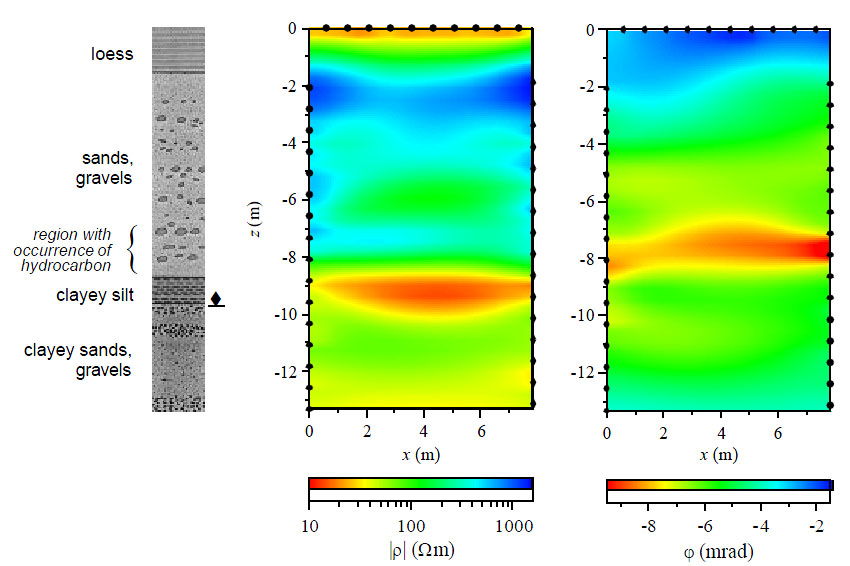
Figure 6. Resistivity and IP responses at a hydrocarbon contaminated site (Slater et al, 2006)
Examples
Example 1 - Groundwater exploration. The majority of
published case histories using IP surveys have been for mining
exploration, but those treating groundwater exploration is
growing: Vacquier, et al. (1957), Kuzmina and Ogil'vi (1965),
Bodmer, et al. (1968), and Sternberg, et al. (1990). Kuzmina
and Ogil'vi reported on work done near the Sauk-Soo River in Crimea
and in the Kalinino region of Armenia. In Crimea, the IP work
consisted essentially of IP sounding (time domain) using the Wenner
array. The alluvial deposits in the studied area were poorly
differentiated by their resistivities, but three horizons were
clearly distinguished by their polarizabilities (figure 6). The
section consisted of a top layer of weak polarizability (h1 = 2-4 m;
η1 = 0.8-1.5%), which represents a dry loamy layer; a second
layer of strong polarizability (h2 = 18-20 m; η2 = 3-5%), which
represented a clayey sand layer saturated with fresh water; and a
third layer of weak polarizability (h3 very thick; η3 = 1%),
which represents impervious siltstones. The survey in this area
demonstrates that the IP work provided more complete information
about the groundwater occurrence than did the resistivity soundings
alone.
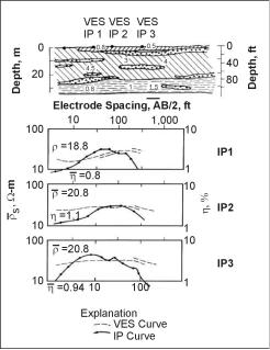
Figure 6. Geoelectric section, VES and IP sounding curves at alluvial deposits. (Zohdy, 1974b).
Example 2 - Detection of metal pipes and cables. Zhang and Luo (1990) show model experiments and analytical results that show that, in certain circumstances, a buried metal pipe or armored cable can introduce anomalies in IP (and apparent resistivity) with large amplitude and wide range. These results are important for two reasons. The first is that such man-made features have the potential to cause "noise" or errors in electrical surveys. The general rule of thumb when planning a survey is to orient soundings and profiles as nearly perpendicular to any known buried pipes or cables as the field conditions allow. The obvious second reason for the importance of this paper is that the IP may be used to locate a pipe or cable. Figure 7 (Zhang and Luo, 1990) shows results of an IP survey using the gradient array in Baima, China. An ηa anomaly of "10% to 3% with a width of more than 200 m was obtained near the road (the dot-and-dash lines on the figure). This anomaly can be traced for 4 km along the road. The trend of the anomalies is basically consistent with road and independent of the stratum strike or structural direction within the prospect area. Apparently, it results from a buried communication cable along the highway rather than geological features. The apparent resistivity profiles (the dot-and-double-dash lines on the figure) also appear to correlate with the cable, but with much less consistency or amplitude.
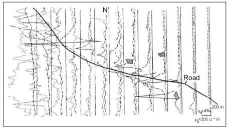
Figure 7. Plan profiles for ηa and ρ a using the gradient array in Baima, China, over a buried cable (Zhang and Luo 1990; copyright permission granted by Society of Exploration Geophysicists).
Example 3 - Mapping soil and groundwater contamination. Cahyna, Mazac, and Vendhodova (1990) show a valuable IP example used to determine the slag-type material containing cyanide complexes that have contaminated groundwater in Czechoslovakia. Figure 8 shows contours of ηa (percent) obtained from a 10-m grid of profiles. The largest IP anomaly (ηa = 2.44%) directly adjoined the area of the outcrop of the contaminant (labeled A). The hatched region exhibits polarizability over 1.5% and probably represents the maximum concentration of the contaminant. The region exhibiting polarizability of less than 0.75% was interpreted as ground free of any slag-type contaminant.

Figure 8. Network of SRP-IP profiles with contours of IP vs ηa (%) and extent of contaminant interpreted on the basis of the geophysical survey. (Cahyna, Mazac and Vendhodova 1990; copyright permission granted by Society of Exploration Geophysicists)
The pages found under Surface Methods and Borehole Methods are substantially based on a report produced by the United States Department of Transportation:
Wightman, W. E., Jalinoos, F., Sirles, P., and Hanna, K. (2003). "Application of Geophysical Methods to Highway Related Problems." Federal Highway Administration, Central Federal Lands Highway Division, Lakewood, CO, Publication No. FHWA-IF-04-021, September 2003. http://www.cflhd.gov/resources/agm/