Environmental Geophysics
Seismic Reflection Methods
The physical process of reflection is illustrated in Figure 1, where the raypaths through successive layers are shown. There are commonly several layers beneath the earth's surface that contribute reflections to a single seismogram. The unique advantage of seismic reflection data is that it permits mapping of many horizon or layers with each shot.. At later times in the record, more noise is present in the record making the reflections difficult to extract from the unprocessed data.
Figure 2 indicates the paths of arrivals that would be recorded on a multichannel seismograph. Note that the subsurface coverage is exactly one-half of the surface distance across the geophone spread. The subsurface sampling interval is one-half of the distance between geophones on the surface. Another important feature of modern reflection-data acquisition is illustrated by figure 3. If multiple shots, S1 and S2, are recorded by multiple receivers, R1 and R2, and the geometry is as shown in the figure, the reflection point for both raypaths is the same. However, the ray paths are not the same length, thus the reflection will occur at different times on the two traces. This time delay, whose magnitude is indicative of the subsurface velocities, is called normal-moveout. With an appropriate time shift, called the normal-moveout correction, the two traces (S1 to R2 and S2 to R1) can be summed, greatly enhancing the reflected energy and canceling spurious noise.
This method is called the common reflection point, common midpoint, or common depth point (CDP) method. If all receiver locations are used as shot points, the multiplicity of data on one subsurface point (called CDP fold) is equal to one-half of the number of recording channels. Thus, a 24-channel seismograph will record 12-fold data if a shot corresponding to every receiver position is shot into a full spread. Thus, for 12-fold data, every subsurface point will have 12 separate traces added, after appropriate time shifting, to represent that point.
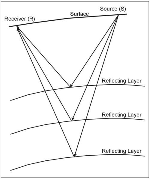
Figure 1. Schematic of the seismic reflection method.
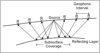
Figure 2. Multichannel recordings for seismic reflection.
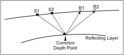
Figure 3. Illustration of common depth point (often called common mid point).
Arrivals on a seismic reflection record can be seen in figure 4. The receivers are arranged to one side of a shot, which is 15 m from the first geophone. Various arrivals are identified on figure 4. Note that the gain is increased down the trace to maintain the signals at about the same size by a process known as automatic gain control (AGC). One side of the traces is shaded to enhance the continuity between traces.
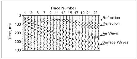
Figure 4. Simple seismic reflection record.
The ultimate product of a seismic reflection survey is a corrected cross section of the earth with reflection events in their true subsurface positions. This section does not present every detail of the acquisition and processing of shallow seismic reflection data. Thus, the difference between deep petroleum-oriented reflection and shallow reflection work suitable for engineering and environmental applications will be stressed.
Cost and frequency bandwidth are the principal differences between the two applications of seismic reflection. One measure of the nominal frequency content of a pulse is the inverse of the time between successive peaks. In the shallow subsurface, the exploration objectives are often at depths of 15 to 45 m. At 450 m/s, a wave with 10 ms peak-to-peak (nominal frequency of 100 Hz) is 45 m long. To detect (much less differentiate between) shallow, closely spaced layers, pulses with nominal frequencies at or above 200 Hz may be required. A value of 1,500 m/s is used as a representative velocity corresponding to saturated, unconsolidated materials because, without saturated sediments, both attenuation and lateral variability make reflection generally difficult.
Common-Offset Seismic Reflection Method
A technique for obtaining one-fold reflection data is called the common-offset method or common-offset gather (COG). It is instructive to review the method, but it has fallen into disuse because of the decreased cost of CDP surveys and the difficulty of quantitative interpretation in most cases. Figure 5 illustrates time-distance curves for the seismic waves that can be recorded. In the optimum offset distance range, the reflected and refracted arrivals will be isolated in time. Note that no quantitative scales are shown as the distances or velocities, and wave modes are distinct at each site. Thus, testing is necessary to establish the existence and location of the optimum offset window. Figure 6 illustrates the COG method. After the optimum offset distance is selected, the source and receiver are moved across the surface. Note that the subsurface coverage is one-fold, and there is no provision for noise cancellation. Figure 7 is a set of data presented as common offset data. The offset between geophone and shot is 14 m. Note that the acoustic wave (visible as an arrival near 40 ms) is attenuated (the shot was buried for this record). Note the prominent reflection near 225 ms that splits into two arrivals near line distance 610 m. Such qualitative changes are the usual interpretative result of a common offset survey. No depth scale is furnished.
Data Acquisition.
A shallow seismic reflection crew consists of three to five persons. The equipment used allows two to three times the number of active receivers to be distributed along the line. A switch (called a roll-along switch) allows the seismograph operator to select the particular set of geophones required for a particular shot from a much larger set of geophones that have been previously laid out. The operator can then switch the active array down the line as the position of the shot progresses. Often the time for a repeat cycle of the source and the archiving time of the seismograph are the determining factors in the production rates. With enough equipment, one or two persons can be continually moving equipment forward on the line while a shooter and an observer are sequencing through the available equipment.
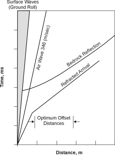
Figure 5. Optimum offset distance determination for the common offset method.
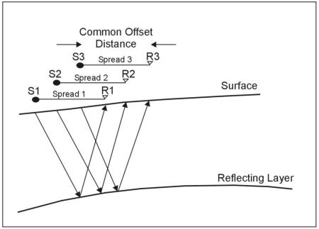
Figure 6. Common offset method schematic.
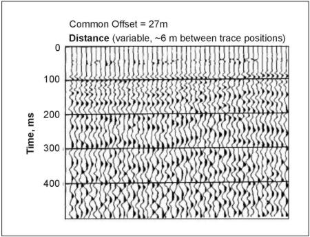
Figure 7. Sample common offset record.
Field data acquisition parameters are highly site specific. Up to a full day of testing with a knowledgeable consultant experienced in shallow seismic work may be required. The objective of these tests is identifiable, demonstrable reflections on the raw records. If arrivals consistent with reflections from the zone of interest cannot be seen, the chances that processing will recover useful data are slim. One useful testing technique is the walkaway noise test. A closely spaced set of receivers is set out with a geophone interval equal to 1% or 2% of the depth of interest - often as little as 30 or 60 cm for engineering applications. By firing shots at different distances from this spread, a well-sampled long-offset spread can be generated. Variables can include geophone arrays, shot patterns, high and low-cut filters, and AGC windows, among others.
Because one objective is to preserve frequency content, table 1 is offered as a comparison between petroleum-oriented and engineering-oriented data acquisition. The remarks column indicates the reason for the differences.
Table 1. Seismic reflection use differences by methodology.
|
|
Petroleum |
Engineering |
Remarks |
|
Explosive seismic source |
10-25 kg or more in a distributed pattern in deep holes |
20 to 50 g, single shot |
To increase frequency content |
|
Mechanical seismic source |
1-7 vibrators 5-15,000 kg peak force 10-100 Hz sweep |
Hammer and Plates, guns |
Cost, increased frequency |
|
Geophones |
Arrays of 12-48 phones; 25-40 Hz fundamental frequency; 3-20 m spacing |
Single or 3-5 geophones 50-100 Hz fundamental frequency; 1-3 m spacing |
To preserve frequency content |
|
Recorders |
Instantaneous floating point, 48-1,000 channels |
Instantaneous floating point, 24-96 channels |
Cost |
|
Passband analog filters |
10-110 Hz |
100-500 Hz |
To increase frequency content |
|
Sample interval |
1-2 ms |
1/4-1/8 ms |
Higher frequencies |
Data Processing
Processing is typically done by professionals using special purpose computers. These techniques are expensive but technically robust and excellent results can be achieved. A complete discussion of all the processing variables is well beyond the scope of this manual. However a close association of the geophysicist, the processor and the consumer is absolutely essential if the results are to be useful. Well logs, known depths, results from ancillary methods, and the expected results should be furnished to the processor. At least one iteration of the results should be used to ensure that the final outcome is successful.
One important conclusion of the processing is a true depth section. The production of depth sections requires conversion of the times of the reflections to depths by derivation of a velocity profile. Well logs and check shots are often necessary to confirm the accuracy of this conversion.
Advantages and Limitations
It is possible to obtain seismic reflections from very shallow depths, perhaps as shallow as 3 to 5 m.
1. Variations in field techniques are required depending on depth.
2. Containment of the air-blast is essential in shallow reflection work.
3. Success is greatly increased if shots and phones are near or in the saturated zone.
4. Severe low-cut filters and arrays of a small number (1-5) of geophones are required.
5. Generally, reflections should be visible on the field records after all recording parameters are optimized.
6. Data processing should be guided by the appearance of the field records and extreme care should be used not to stack refractions or other unwanted artifacts as reflections.
A variant of seismic reflection used at the surface of water bodies is subbottom profiling or imaging. The advantage of this technique is the ability to tow the seismic source on a sled or catamaran and to tow the line of hydrophones. This procedure makes rapid, continuous reflection soundings of the units below the bottom of the water body, in other words, the subbottom. This method and significant processing requirements have been recently developed by Ballard, et al., (1993) of the U.S. Army Engineer Waterways Experiment Station (WES). The equipment, acquisition, and processing system reduce the need for over-water boring programs. The developed WES imaging procedure resolves material type, density, and thickness (Ballard, et al., 1993).
Basic Concepts
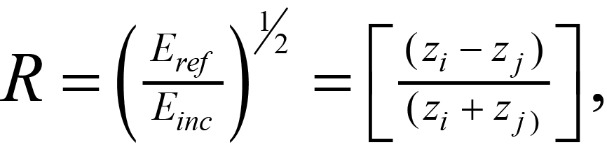
The acoustic impedance method may be used to determine parameters of the soft aqueous materials. The acoustic impedance z for a unit is the product of its pb and VP. The reflection coefficient R from a particular horizon is
 (7)
(7)
where
Erefl = energy reflected at the i-j unit boundary
Einc = incident energy at the i-j unit boundary
zi = acoustic impedance of the i (lower) material
zj = acoustic impedance of the j (upper) medium
At the highest boundary, the water-bottom interface, z j ,water is known to be 1.5 * 10 9 g/(m 2 s). Since the E ref l , 1-2 can be determined, and E inc , 1-2 and z 1,water are known, z i , 2 may be determined. V P , 2 may be assessed from the depth of the 2-3 boundary, and thus ? i , 2 may be resolved. The material properties of lower units can be found in succession from the reflections of deeper layers.
Data Acquisition
A variety of different strength sources are available for waterborne use. By increasing strength, these sources are: pingers, boomers, sparkers, and airguns. Although there is some strength overlap among these sources, in general, as energy increases, the dominant period of the wave increases. For the larger source strength, therefore, the ability to resolve detail is impaired as period and wavelength become larger. The resolving accuracy of the system may change by more than an order of magnitude from <0.2 m for a pinger to >1.0 m for an airgun.
The conflicting impact of energy sources is the energy available for penetration and deeper reflections. The greater energy content and broad spectrum of the boomer allow significantly greater depth returns. Some near-bottom sediments contain organic material that readily absorbs energy. Higher energy sources may allow penetration of these materials.
Data collection is enormous with a towed subbottoming system. Graphic displays print real-time reflector returns to the hydrophone set. Recording systems retrieve the data for later processing. The field recorders graph time of source firing versus time of arrival returns. Figure 8 provides the field print for Oakland Harbor (Ballard, McGee, and Whalin, 1992).
Data Processing
Office processing of the field data determines the subbottoming properties empirically. The empiricisms are reduced when more sampling (boring) data are available to assess unit ρ and loss parameters for modeling. The processing imposes the Global Positioning System (GPS) locations upon the time of firing records to approximately locate the individual shot along the towed boat path. The seismic evaluation resolves the layer VP and unit depths. From the firing surface locations and unit depths, the field graphs are correlated to tow path distance versus reflector depths. Figure 257 shows cross sections of the Gulfport Ship Channel, Mississippi. These are fence diagrams of depth and material types once all parallel and crossing surveys are resolved.
Advantages and Limitations
The subbottoming technique can be applied to a large variety of water bodies. Saltwater harbors, shipping channels, and river waterways were the original objective for the technique. The method is now used on locks, dams, reservoirs, and engineering projects such as the location of pipelines.
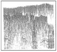
Figure 8. Reflected subbottoming signal amplitude cross section, 3.5 kHz in Oakland Harbor, California. (Ballard, McGee and Whalin, 1992)
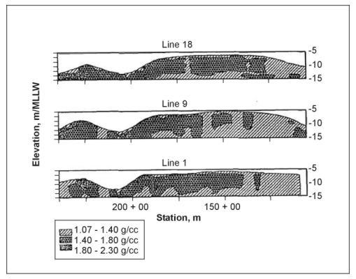
Figure 9. Density cross section in Gulfport ship canal, Mississippi. (Ballard. McGee and Whalin 1992)
Basic Concepts
Fathometers are also called Echo Sounders and are similar to reflection seismic profilers in that they also employ an acoustic source and receiver placed immediately beneath the surface of the water. However, fathometers differ from reflection seismic profilers in that they use higher frequency acoustic source pulses varying from less than 10 kHz up to about 200 kHz. Some of this energy transmitted by the source is reflected from the sediments at the water bottom, and the reflections are recorded by the receiver and stored digitally.
Data Acquisition
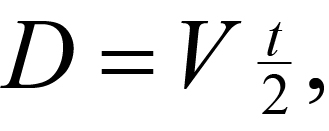
Fathometers determine water depth by repeatedly transmitting seismic energy through the water column and recording the arrival time of the reflected energy from the water bottom. The time required for the seismic signal to travel from its source to a reflector and back is known as the two-way travel time, and it is measured in milliseconds (ms) (equal to 1 x 10⁻³ seconds). The Fathometer calculates the depth to a water bottom by dividing the two-way travel time by two and multiplying the result by the velocity of sound through water:
 (8)
(8)
where
D= depth to the water bottom (m),
V= velocity of sound through water (m/s), and
t= two-way travel time (s).
Fathometer surveys are conducted while traveling at a moderate speed in a boat. Typically, the transducer is mounted on the side of the boat and placed in the water. Data recording is essentially automatic with a t recorder plotting providing a hard copy of the data or a computer screen may be used for the display. The data may also be stored on magnetic tape for further processing and plotting. As with the CSP method, GPS can be used to position the data.
Data Processing
The depth value is printed as a continuous graphic profile and/or displayed as a numeric value by the Fathometer. Fathometers are calibrated by adjusting the value of V, which may vary slightly depending on water type. Most Fathometers use a narrow-bandwidth 200 kHz seismic signal. These Fathometers provide accurate depth data, but little or no information about the subbottom. Fathometers that use a lower frequency signal, such as 20 kHz, can detect reflected energy from subbottom interfaces, such as the bottom of an infilled scour hole.
Fathometer systems come with black and white t recording systems and in color systems. Colors are often assigned according to the different amplitudes of the reflected signals. Fathometers color step sizes as low as four dB are now available, allowing quite small changes in the reflected signals to be observed. An event marker button is often available allowing vertical line marks to be placed on the records when specific locations are selected by the operator. Sometimes the data can be downloaded to a computer allowing digital processing to be done along with data plots.
A color Fathometer can be calibrated to measure and display in color the amplitude of the reflected signal, which, in constant water depths, can be related to characteristics of the bottom material.
Data Interpretation
Traces from adjacent source/receiver locations are plotted side-by-side to form an essentially continuous time-depth profile of the stream bottom. Estimated seismic interval velocities can be used to transform the time-depth profile into a depth profile. However, water velocities are a function of suspended sediment load, and can vary appreciably.
The data are interpreted by viewing the plotted data. The response of specific objects may be used if these were noted on the records using a button marker.
Figure 10 shows Fathometer data recorded with a 200 kHz transducer. Note that only the water depth is observed in these data. Because of the high frequency, little energy is transmitted into the bottom sediments, and thus no reflections are observed from within the sediments.
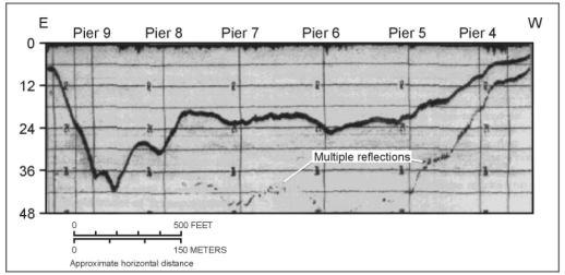
Figure 10. Fathometer data recorded with 200 kHz transducer. (Placzek, et al. 1995, USGS Report 95-4009)
Figure 11 presents fathometer data using a 3.5 kHz transducer. Because of the lower frequency, some of the energy is transmitted into the sediments and reflections are seen.
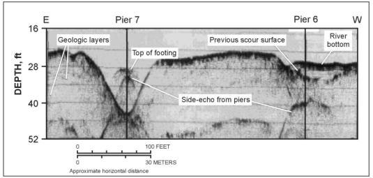
Figure 11. Fathometer data recorded using a 3.5 kHz transducer. (Placzek, et al. 1995, USGS Report 95-4009)
Advantages and Limitations
The main advantages of Fathometers (in continuous mode) are as follows:
1. The tool can provide an accurate depth-structure model of the water bottom (if acoustic velocities are known).
2.
Post acquisition processing (migration) can be applied.
The main disadvantages of Fathometers (in continuous mode) are as follows:
1. The source and receiver need to be submerged. Profiles cannot be extended across emerged sand bars or onto the shore.
2. The equipment is relatively expensive (hardware and software).
3. Data may be contaminated by noise (multiple reflections, and echoes from the shoreline, water bottom, and/or piers).
4. Post acquisition processing (migration) may be required in areas where significant structural relief is present.
Fathometers are also employed in a spot survey mode. In this type of survey, sounding data (single reflection traces) are acquired at irregularly (or uniformly) spaced intervals (typically on the order of meters) at the water surface. The first high-amplitude reflected event is usually interpreted to be the water bottom reflection. Note, that spot data usually cannot be accurately migrated because of aliasing problems.
The pages found under Surface Methods and Borehole Methods are substantially based on a report produced by the United States Department of Transportation:
Wightman, W. E., Jalinoos, F., Sirles, P., and Hanna, K. (2003). "Application of Geophysical Methods to Highway Related Problems." Federal Highway Administration, Central Federal Lands Highway Division, Lakewood, CO, Publication No. FHWA-IF-04-021, September 2003. http://www.cflhd.gov/resources/agm/