
Geophysical Methods
Ground Penetrating Radar
Ground penetrating radar (GPR) is a shallow, high-resolution geophysical method that uses high-frequency, pulsed, electromagnetic waves to image the subsurface. A GPR unit transmits electromagnetic energy into the ground which is reflected, refracted, or scattered back to the surface depending on the features it encounters (such as changes in geologic media or buried objects). Typically GPR is limited to depths of approximately 10 meters, but in highly resistive subsurface materials, such as salt or ice, depths of 100s of meters may be possible (Everett, 2013). High-frequency antennas (200-400 MHz range) can achieve resolutions of a few centimeters at shallow depths, while low-frequency antennas (50 MHz or less) may have a resolution of approximately one meter at greater depths (Everett, 2013). As with most geophysical techniques, the results are non-unique and should be compared with direct physical evidence, such as trench or boring data (Everett, 2013). Integration of GPR data with other surface geophysical methods, such as seismic, resistivity, or electromagnetic methods, reduces uncertainty in site characterization.
Typical Uses
GPR is commonly used for environmental, engineering, archeological, and other high-resolution shallow investigations. It can be used to map subsurface features such as depth to bedrock, depth to the water table, depth and thickness of soil and sediment strata (including under freshwater bodies), buried stream channels, and the location of cavities and fractures in bedrock. Other applications include locating objects such as pipes, drums, tanks, cables, buried waste, or buried utilities; mapping landfill and trench boundaries; and mapping contaminated groundwater (Benson et al., 1984; U.S. EPA, 1993).
↩Theory of Operation
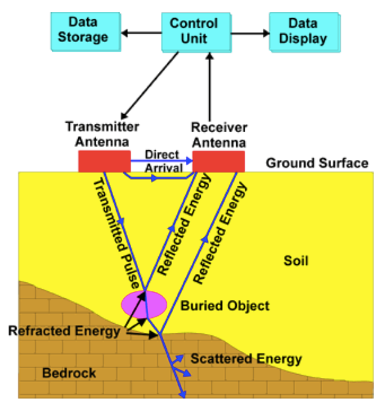
Figure 1. An electromagnetic pulse is emitted from a transmitter antenna. When the wave encounters a layer or object with different electrical properties, part of the energy is reflected back toward the surface where a receiver antenna records the signal (ASTM, 2019).
GPR uses a transmitter antenna to send high-frequency, pulsed, electromagnetic waves (typically from 10 MHz to 1,000 MHz; commercially available units can go up to 7000 MHz [ASTM 2019]) into the subsurface to acquire information. The wave spreads out and travels downward until it hits a buried object or boundary (e.g., a different geologic unit) with different electromagnetic properties (Figure 1). Part of the wave energy is reflected or scattered back to the surface, while part of the energy continues to travel downward. The wave is reflected back to the surface to a receiver antenna that records the amplitude of the reflected energy and the arrival time of the wave on a digital storage device (Benson et al., 1984; U.S. EPA, 1993).
Electromagnetic waves travel at a velocity that is determined primarily by the electrical permittivity1 of the material. The velocity of the electromagnetic wave is different between materials with different electrical permittivity, and a signal passed through two materials with different permittivities over the same distance will arrive at different times. The time that it takes for the wave to travel from the transmitter antenna to the receiving antenna is called the transit time (measured in nanoseconds ns, where 1 ns=10-9 s) and is proportional to the depth of the buried object or target layer. Since the velocity of an electromagnetic wave in air is 0.3 m/ns, the travel time for an electromagnetic wave in air is approximately 3.3 ns/m traveled. The electromagnetic wave velocity in a non-magnetic medium is proportional to the inverse square root of the permittivity of the material (Everett, 2013).
$$ V=C / \sqrt{\epsilon_r} $$
Where:
V = velocity of the material (m/ns)
C = the speed of light in a vacuum (3 x 10⁸ m/s)
\( {\epsilon_r} \) = relative dielectric permittivity
Since the permittivity of earth materials is always greater than the permittivity of air (Table 1), the travel time of a wave in a material other than air is always greater than 3.3 ns/m. The depth of the object or target layer can be calculated using this velocity by the equation (Benson et al., 1984):
$$ D=\frac{C T}{2 \sqrt{\epsilon_r}}=\frac{V_m T}{2} $$
Vm = velocity of the material (m/ns)
C = the speed of light in a vacuum (3 x 10⁸ m/s)
\( {\epsilon_r} \) = relative electrical permittivity (dielectric constant)
T = two-way travel time in nanoseconds
Table 1. Electromagnetic Properties of Various Earth Materials
| Material | Relative Permittivity | Wave Velocities (m/Ns) | Conductivity (mS/m) |
|---|---|---|---|
| Air | 1 | 0.3 | 0 |
| Fresh water | 80 | 0.033 | 0.5 |
| Sea water | 80 | 0.01 | 3,000 |
| Sand (dry) | 3-5 | 0.15 | 0.01 |
| Sand (wet) | 20-30 | 0.06 | 0.1-1 |
| Silts | 5-30 | 0.07 | 1-100 |
| Clays | 5-40 | 0.06 | 2-1,000 |
| Ice | 3-4 | 0.16 | 0.01 |
| Granite | 4-6 | 0.13 | 0.01-1 |
| Limestone | 4-8 | 0.12 | 0.5-2 |
Adapted from Table 4-3 from USACE, 1995.
↩System Components
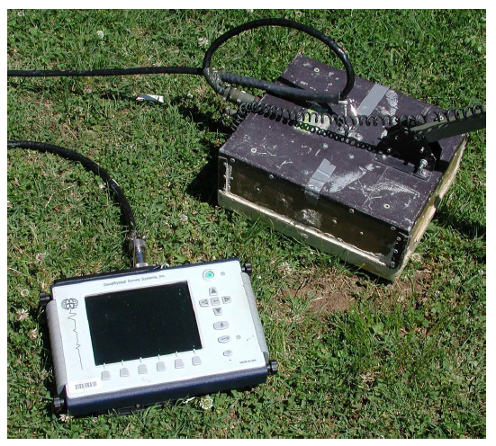
Figure 2. An example of a GPR system with the antenna separate from the electronics and computer controls. The system can be towed by hand or mounted on a cart (Lucius et al., 2006).
GPR equipment for measuring subsurface conditions normally consists of a radar control unit that also records data, one or two antennas for transmitting and receiving, a power source, cables, and data storage and display devices (Figure 2). One to two people can manage the equipment and survey (Lucius et al., 2006).
The transmitter antenna converts electrical currents into electromagnetic waves that propagate into the material. The receiver antenna captures the reflected electromagnetic waves and converts them into current. The control unit records the reflected wave data.
Antennas come in various sizes with larger sizes having lower frequencies. Lower frequencies are used to detect layers or objects at greater depths (15-20 meters); however, the spatial resolution is lower (0.5-1.5 meters). Mid-sized antennas can reach depths of 3 to 6 meters. The depth of investigation depends on the electrical conductivity and dielectric permittivity of the subsurface. High electrical conductivity (for example, highly conductive clays) or dielectric permittivity attenuate electromagnetic waves. If it is assumed that the desired spatial resolution is approximately 25% of the target depth, Table 2 can be used as a guide for selecting a frequency to use in the survey (Annan, 2001, as cited by Robinson et al., 2013). At frequencies close to 100 MHz, a resolution of 1 meter can be achieved.
Table 2. Frequency Values Guideline
| Depth (m) | Center Frequency (MHz)* |
|---|---|
| 0.5 | 1,000 |
| 1.0 | 500 |
| 2.0 | 200 |
| 5.0 | 100 |
| 10.0 | 50 |
| 30.0 | 25 |
| 50.0 | 10 |
*If the desired spatial resolution is 25% of the target depth.
Adapted Annan, 2001, as cited by Table 3 of Robinson et al., 2013
GPR systems are digitally controlled, and data are usually digitally recorded for post-survey processing and display. The digital control and display generally consist of a microprocessor, memory, and a mass storage medium to store the field measurements. A small micro-computer and standard operating system often are used to control the measurement process, store the data, and serve as a user interface.
↩Modes of Operation
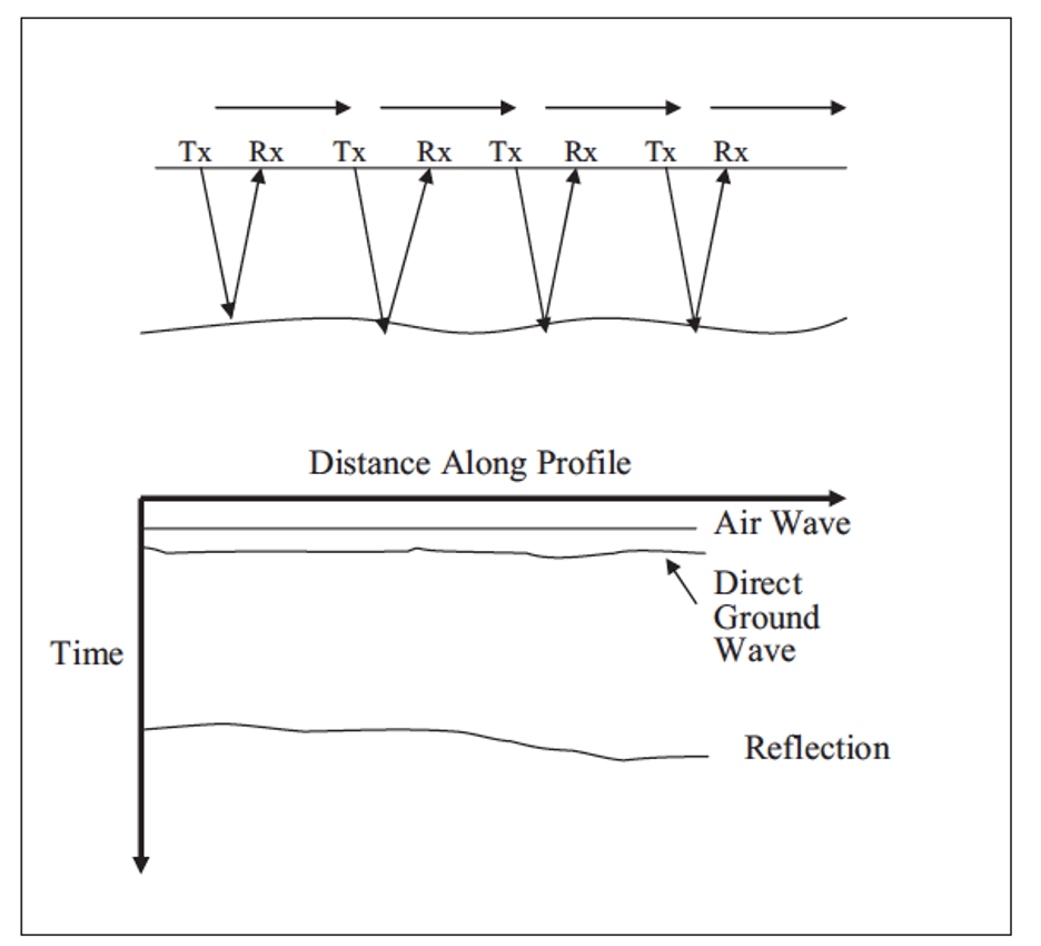
Figure 3. A generalized schematic showing the common offset configuration for reflective profiling (top) and idealized wave arrivals (bottom). The separation distance (s) between the transmitter and receiver is kept constant as the GPR unit is moved from station location to station location collecting measurements (Baker, et al., 2007).
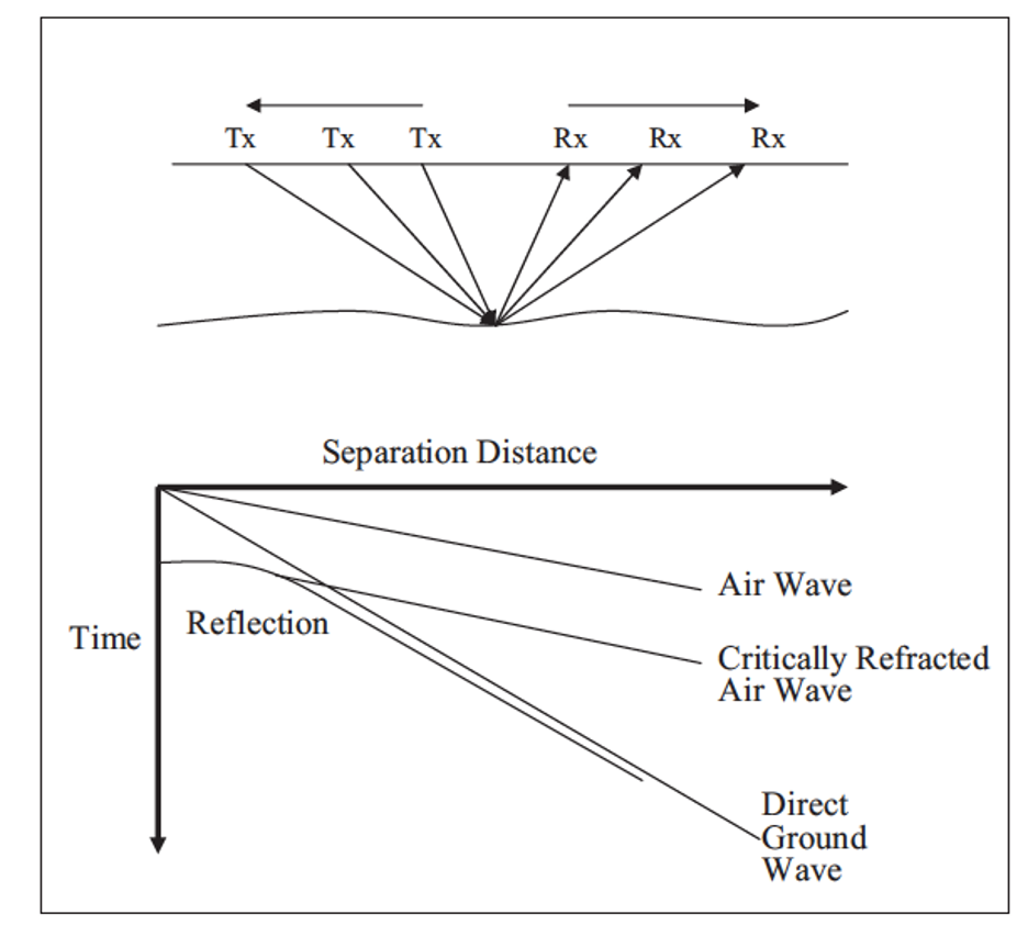
Figure 4. A generalized schematic showing the common midpoint configuration for the reflective profiling mode (top) and idealized wave arrivals (bottom). The transmitter (T) and receiver (R) are moved symmetrically away from a fixed midpoint to collect sequential measurements at the station location (Baker, et al., 2007).
GPR data can be collected by deploying the equipment at the ground surface, in a borehole, on a boat or platform in low-conductivity2 water, or from a plane or drone.
There are several configurations of transmitter and receiver antennas that may be used for surface or borehole data collection. The most common configuration is referred to as the Reflection Profiling Method and includes common offset and common midpoint configurations. In the common offset configuration (Figure 3), radar waves are transmitted, received, and recorded each time the transmitting and receiving antenna pair moves a fixed distance. In the common midpoint configuration (Figure 4), the transmitter and receiver antenna must be capable of being separated. Data are collected at increasing distances around a midpoint. In general, the common offset configuration of the transmitter and receiver antenna is used when collecting GPR data by boat/platform or by plane or drone.
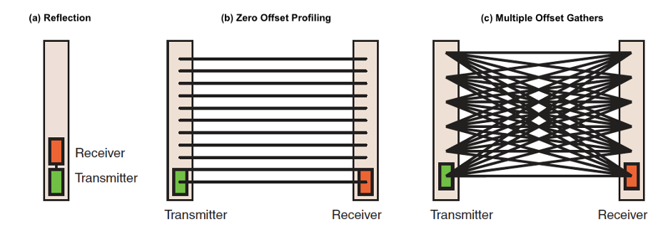
Figure 5. Example configurations of receivers and antennas in borehole GPR data collection. (Johnson and Joesten, 2005).
Borehole applications have several possible configurations of transmitting and receiving antennas. One configuration includes a transmitter and receiver separated by a set distance that is lowered into a single borehole (Figure 5a). In cross-borehole configurations, the transmitting and receiving antennas can be configured for either the Zero-Offset Profiling (ZOP) or the Multiple-Offset Gathers. In ZOP (Figure 5b), both the receiver and transmitter antennas are lowered to equal, predetermined depths before a measurement is made, and the process is repeated over the depth of interest. In a Multiple-Offset Gathers (Figure 5c), the transmitter is held at a predetermined depth in one borehole while the receiver(s) is lowered in regular steps down the other borehole(s). After the receiver(s) collects data over the depth of interest, the transmitter is lowered to the next interval, and the process is repeated until the transmitter reaches the depth of interest. The readings are then manipulated to provide a detailed 2-D depiction of the subsurface between the boreholes (Annan, 2005; Kayen, 2000).
Surface Mode
For surface applications of GPR, the transmitting and receiving antennas are separated by a set distance and can be mounted either on a handheld device (Figure 6), on a cart (Figure 7a) or sled towed by hand (Figure 7b), or vehicle (Figure 7c) along the ground in a sampling grid or along a transect.
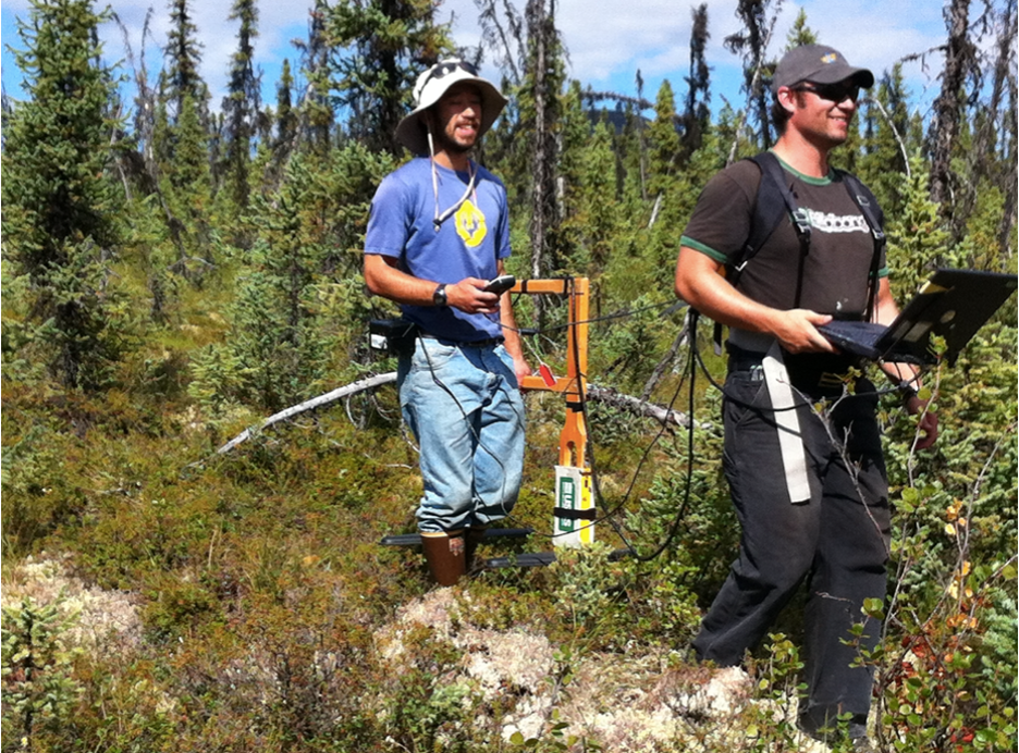
Figure 6. GPR data are collected with handheld equipment. The lead individual carries the electronic equipment while the second person carries the receiving antennas (USGS).
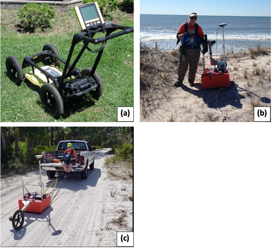
Figure 7. GPR equipment with: (a) Antenna and electronics mounted between the cart's wheels with monitor and computer controls mounted on the handle (Lucius et al., 2006); (b) antenna mounted on a sled and towed by hand (USGS); and (c) towed behind a truck along a transect (USGS).
Borehole Mode
As discussed above and depicted in Figure 5, borehole GPR equipment can be deployed either in a single borehole or cross-hole with various configurations of transmitter and receiver antenna. Figure 8 shows the cross-hole mode of deployment where a transmitter is deployed in one well, and the receiver is deployed in a second well.
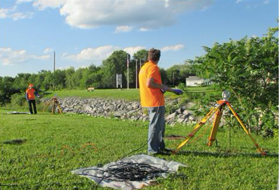
Figure 8. Cross-hole collection of GPR data; a receiver is deployed down one well and a transmitter is deployed down an adjacent well (USGS).
Aerial and Watercraft Mode
The depth of investigation depends on the electrical conductivity and dielectric permittivity of the subsurface. High electrical conductivity (for example, highly conductive clays) or dielectric permittivity attenuate electromagnetic waves.
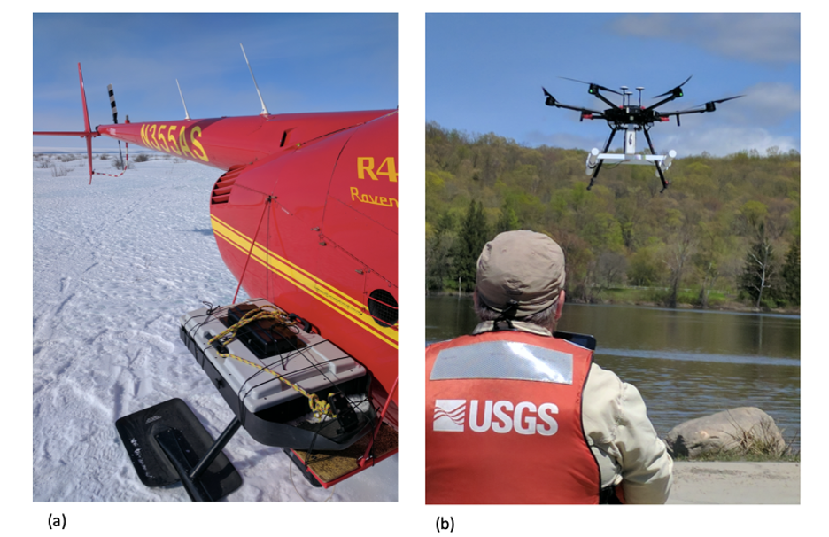
Figure 9. A helicopter (a) and drone (b) equipped with GPR instruments (USGS).
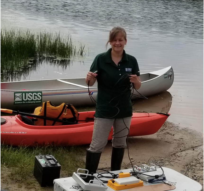
Figure 10. Connecting power and data cables on a GPR system to set up the equipment to collect data from a canoe and kayak (USGS).
Data Display and Interpretation
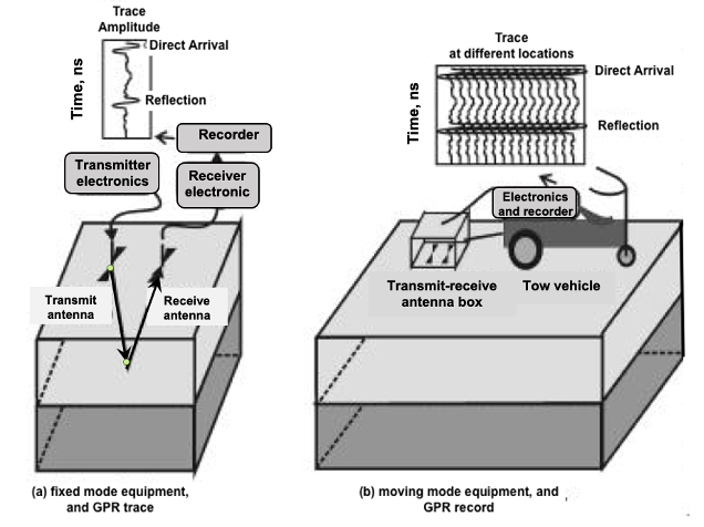
Figure 11. A generalized schematic of (a) a one-dimensional trace collected at a single station location, and (b) a time-distance wiggle trace from multiple station locations along a survey transect (Daniels 2000).
The objective of GPR data presentation is to display the processed data in an image that approximates the subsurface, including anomalies in their proper spatial positions. The most common display of GPR data, referred to as a trace, shows amplitude versus the two-way travel time (ns). A single GPR trace consists of the transmitted pulse followed by pulses that are reflected from objects or layers (Figure 11a). Several traces from the same location are typically stacked and averaged to provide better resolution of weaker reflections. When traces from along the survey transect are placed side by side, they create a GPR cross section or time-distance record that depicts a pseudo-image of the subsurface (Figure 11b). If the permittivities of the subsurface media are known, the two-way time of travel can be converted to depth using the equation3 in Theory of Operation (Daniels 2000![]() ).
).
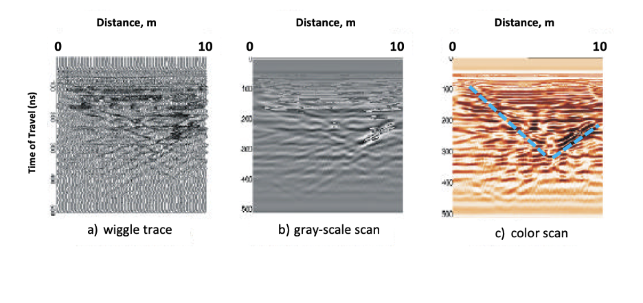
Figure 12. Examples of 2-D GPR data displays include (a) wiggle traces composed of individual one-dimensional traces; (b) gray-scale scans in which values have been assigned to the range of amplitudes; and (c) color scans, in which a color scale is assigned to the range of amplitude. The change in the scan highlighted by the dashed blue line could be indicative of subsurface structures such as a buried trench or a buried stream channel. The vertical axis is the two-way time of travel in ns, and the horizontal axis is the surface position in meters. (Daniels 2000![]() ).
).
Displays of surface GPR data include: (1) one-dimensional (1-D) trace (single trace); (2) two-dimensional (2-D) cross section; and (3) 3-D display. A 2-D cross section, or wiggle trace, is composed of multiple adjacent 1-D traces (Figure 12a). The two-way travel time is plotted on the vertical axis, and the surface position is on the horizontal axis. When many traces are measured along a survey transect, the wiggle trace may be unclear. In these instances, the data are converted to a 2-D scan display by assigning a color or gray-scale to the amplitude (Figure 12b and 12c). Borehole data can also be displayed as a 2-D cross section (Daniels 2000![]() ).
).
Data are usually recorded along profile lines in a continuous recording system, or at discrete points. Multiple 2-D line scans can then be combined to build a 3-D display of the subsurface (Figures 13 and 14). The 3-D blocks can be viewed from any angle as a solid block or as block slices (Daniels 2000![]() ). The accurate location of each trace is critical to producing accurate 3-D displays. 3-D block views can be constructed in a variety of ways, such as a solid block or as block slices (Figure 14) (Daniels 2000
). The accurate location of each trace is critical to producing accurate 3-D displays. 3-D block views can be constructed in a variety of ways, such as a solid block or as block slices (Figure 14) (Daniels 2000![]() ).
).
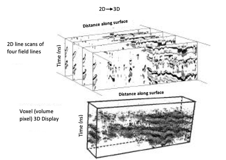
Figure 13. An example of building a 3-D display from a series of 2-D cross sections (Daniels 2000![]() ).
).
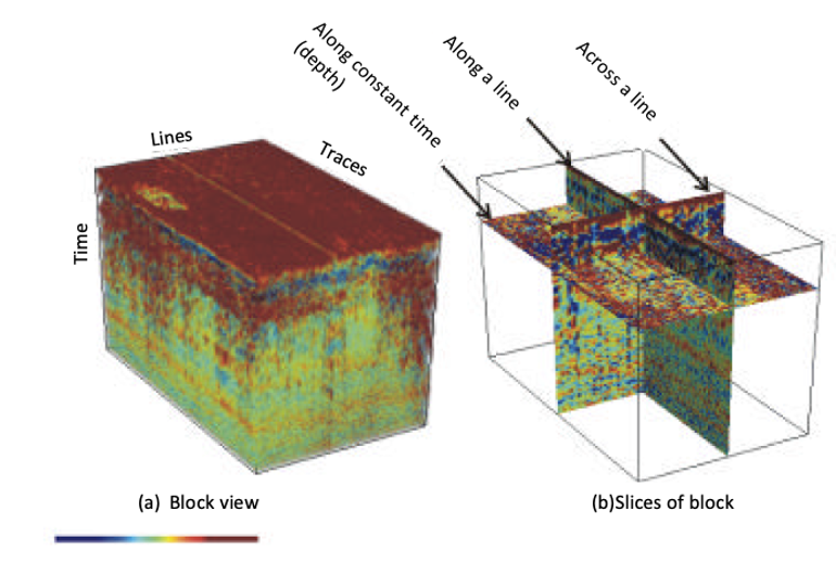
Figure 14. A depiction of (a) block view display of 3-D GPR data, and (b) dissecting the 3-D block into slices (Daniels 2000![]() ).
).
Data display is an integral part of data interpretation. In general, targets of interest are easier to identify and isolate on 3-D data sets than on conventional 2-D profile lines. Simplifying the image by eliminating noise is the most important factor for interpretation. Image simplification may be achieved by:
- Carefully assigning the amplitude-color ranges.
- Displaying only one polarity of the GPR signal.
- Decreasing the size of the data set that is displayed as the complexity of the target increases.
- Carefully selecting the viewing angle.
Further image simplification in cases involving very complex (or multiple) targets may also be achieved by displaying only the peak values (maximum and minimum values) for each trace.
Performance Specifications
The performance of the GPR method depends upon the site-specific surface and subsurface conditions. Performance specifications include the parameters listed in Table 3.
Table 3. Performance Specifications for GPR
| Parameter | Unit of Measure | Typical Range |
|---|---|---|
| Frequency | Megahertz (MHz) | High-frequency antennas: 500-1,000 MHz Low-frequency antennas: 10-125 MHz |
| Electrical Conductivity | milliSiemens per meter (mS/m) | 0-1000* |
| Relative Permittivity | Dimensionless | 0-80* |
| Dynamic Range | Decibels (dB) | 90-130 |
| Depth of Investigation | Meters | 1-10s |
| Resolution | Meters | Low-frequency antennas: ~ 1 meter High-frequency antennas: ~0.1 meters |
(Benson, et al., 1984 and USACE, 1995)
Frequency
The frequency of the antenna used affects the resolution of the GPR profile and the attenuation of the radar signal. Resolutions of just a few centimeters can be obtained by using a higher frequency antenna (500-1000 MHz). However, higher frequencies provide less penetration (depth) with higher resolution. Lower frequencies (10-125 MHz) provide greater penetration depth with less resolution; objects or features smaller than one meter are unable to be defined.
Electrical Conductivity
The electrical conductivity of the subsurface materials is a factor in the attenuation of the radar signal emitted by the GPR antenna. Materials with higher conductivities will result in greater attenuation of the signal.
Relative Permittivity
Relative permittivity, or a materials dielectric constant, is based on how easily a material becomes polarized by the imposition of an electric field. It is a dimensionless number. Values range from one for air to 80 for both fresh water and sea water. Most GPR reflections are due to changes in the relative permittivity of materials (subsurface layers or buried objects). The greater the change in permittivity, the more signal is reflected. In addition to having a sufficient electromagnetic property contrast, the boundary between the two materials needs to be sharp.
Areas with subsurface contamination often have very different permittivities than uncontaminated areas. GPR has been used to map highly conductive contaminated groundwater plumes (Porsani et al., 2004; Pomposiello et al., 2004![]() ). Also, studies have shown that weathered fuel releases create a "halo" of conductive soil and groundwater around them that are detectable by GPR (Sauck et al., 1998; Atekwana et al., 2002; Bradford, 2003). Non-aqueous phase, non-polar organic contaminants, such as fuels and chlorinated solvents, generally have very low permittivities. In theory, these should provide a good contrast, and studies have shown that GPR can track their movement in the subsurface during a controlled release (Sneddon et al., 2000; Brewster et al., 1995); however, in practice, differentiating relatively thin layers of free product from other reflectors, where the release area is unknown, has not been successful. Studies suggest that GPR can aid remediation monitoring by tracking changes in the subsurface conditions (Lane et al. 2004, Paterson, 1997
). Also, studies have shown that weathered fuel releases create a "halo" of conductive soil and groundwater around them that are detectable by GPR (Sauck et al., 1998; Atekwana et al., 2002; Bradford, 2003). Non-aqueous phase, non-polar organic contaminants, such as fuels and chlorinated solvents, generally have very low permittivities. In theory, these should provide a good contrast, and studies have shown that GPR can track their movement in the subsurface during a controlled release (Sneddon et al., 2000; Brewster et al., 1995); however, in practice, differentiating relatively thin layers of free product from other reflectors, where the release area is unknown, has not been successful. Studies suggest that GPR can aid remediation monitoring by tracking changes in the subsurface conditions (Lane et al. 2004, Paterson, 1997 ![]() , and Bradford, 2004).
, and Bradford, 2004).
Dynamic Range
The dynamic range or performance figure of a specific GPR system represents the total attenuation loss during the two-way transit of the radar signal that still allows reception of the reflected signal. Attenuation losses above the dynamic range will cause the signal to become undetectable. Attenuation is defined by the equation:
$$ \alpha=1.69 \sigma / \epsilon^{\frac{1}{2}} $$
Where:
\( \alpha \) = attenuation in decibels/m (dB/m)
\( \sigma \) = electric conductivity in mS/m
\( \epsilon \) = dielectric constant (dimensionless)
For a material such as a clay that has an electrical conductivity of 100 mS/m and some water content (\( \epsilon \) =20), the attenuation in decibels/m would be:
\( \alpha \) = 1.69(100 mS/m)/200.5 = 38 dB/m
If the GPR system has a dynamic range of 100 dB, then the radar signal would be attenuated in 2.6 meters of travel.
Depth of Investigation
The principal factor limiting the depth of GPR investigation is attenuation of electromagnetic waves in subsurface materials. Depth of penetration is commonly less than 10 meters in most soil and rock, although penetration in conductive clays (e.g., smectites) and in materials having conductive pore fluids may be less than one meter (Benson et al., 1984). On the other hand, depth of penetration can be more than 30 meters in water-saturated sands, while depths of up to 100s of meters in highly resistive materials, such as ice, may be possible (Everett, 2013).
Resolution
GPR provides the highest lateral and vertical resolution of any surface geophysical method. Various frequency antennas (10 to 1,000 MHz, though commercially available units can go up to 7,000 MHz [ASTM, 2019]) can be selected to collect appropriate data to meet project needs. Lower frequency provides greater penetration with less resolution. Higher frequencies provide less penetration with higher resolution. Resolution of a layer or anomaly a few centimeters thick can be obtained with high-frequency (1 GHz) antennas at shallow depths, while lower frequency antennas (100 MHz) may have a resolution of approximately one-meter thickness at greater depths. Horizontal resolution is determined by the distance between station measurements, and/or the sample rate, and the towing speed of the antenna.
Additionally, the following factors should be considered when conducting a GPR survey:
Interferences - GPR is sensitive to "noise" or unwanted reflections or scattering caused by various geologic and anthropogenic factors. Geologic noise can be caused by boulders, animal burrows, tree roots, and other inhomogeneities that cause unwanted reflections or scattering. Anthropogenic noise can be caused by nearby vehicles, buildings, fences, power lines, and trees. Shielded antennas can limit some of these unwanted reflections. Electromagnetic transmissions from cellular telephones, two-way radios, televisions, and radio and microwave transmitters may also cause noise on GPR records (Benson et al., 1984).
Calibration - The manufacturer's recommendations should be followed for the calibration and standardization of GPR equipment. An operational check should be conducted before each project and before starting fieldwork each day. A routine check of equipment should be made on a periodic basis and after any problem encountered with the equipment.
Quality Control - Quality control can be applied to the acquisition, processing, and interpretation phases of the survey. Good quality control requires following standard procedures (e.g., those provided in ASTM Standard Guide D6432-19) and appropriate documentation.
Precision - Precision is defined as the repeatability of measurements. Factors affecting precision include the location of the antennas, tow speed, coupling of the antennas to the ground surface, variations in soil conditions, and ability and care involved in choosing reflections. Repeatability of GPR measurements can be 100% if soil conditions remain the same (e.g., soil moisture) (ASTM, 2019).
Accuracy - The accuracy of depth to target determinations is dependent on how precisely travel time is related to the actual depth units. The velocity (two-way travel time per unit distance) of the specific subsurface layers at the site must be determined. Table 1 lists velocities for natural materials ranging from six to 40 nanoseconds per meter (ns/m). In addition to choosing appropriate travel times, accuracy is also affected by equipment positioning differences, and proper attention to processing, interpretation, and site-specific conditions.
↩Advantages
Advantages of using GPR include (Benson et al., 1984; Wightman et al., 2003):
- GPR measurements are non-intrusive and relatively easy to collect.
- GPR provides the highest lateral and vertical resolution of any surface geophysical method.
- Antennas may be pulled by hand, with a vehicle from 0.8 to 8 kph, or more.
- GPR data can often be interpreted in the field without data processing.
- Graphic displays of GPR data often resemble geologic cross sections.
- When GPR data are collected on closely spaced (less than one meter) lines, these data can be used to generate 3-D views that significantly improve interpretation of subsurface conditions.
- GPR can be used on paved or unpaved surfaces and in boreholes with various casings.
Limitations
Limitations of using GPR in site investigations include (Benson et al., 1984; Lucius et al., 2006):
- The presence of trees or vegetation may affect the ability to collect measurements in a line or grid for cross-section or 3D views.
- The depth of penetration may be limited by the presence of conductive clays or high-conductivity pore fluid.
- Interpretation of GPR data requires a trained operator.
- GPR can be susceptible to electromagnetic noise.
Cost
The cost of GPR systems varies widely depending on the complexity of the systems. Most systems fall in the $15,000 to $50,000 (USD) range. GPR systems can be rented for about $1,000 (USD) per week and a $300 (USD) mobilization charge. GPR surveys can be conducted by contractors with costs ranging from $1,000 to $2,000 (USD) per day depending on data interpretation needs and if a report is required.
↩Case Studies
GPR For Earth and Environmental Applications: Case Studies From India
Sonkamble, S. and S. Chandra, Journal of Applied Geophysics, Volume 193, October
2021.
A GPR survey using Terra Sirch-3000 single channel control GPR meter with 2D data collection was performed for civil engineering, environmental, archeological, geological features, aquifer contamination, and sea water intrusion studies. The scanned images were verified with excavations, electrical resistivity tomography, and soil and water chemistry, which complemented the GPR anomalies. Results helped to: 1) identify caving in trenchless MS pipe; 2) discover an ancient temple; 3) decipher a subsurface intrusive body; 4) detect clandestine pipes; 5) demarcate fresh groundwater zones within industrial clusters; and 6) identify sea water intrusion in coastal area.
One-off Geophysical Detection of Chlorinated DNAPL During Remediation of an Industrial Site: A Case Study
Fiorentine, E., et al., AIMS Geosciences, Vol 7(1), 1-21 pp., January 2021.
A geophysical survey was performed on an industrial site to find the precise location of chlorinated DNAPL for treatment of the saturated zone. As the excavation neared the saturated zone, geophysical measurements were conducted at the bottom of the pit. Whereas electrical resistivity tomography measurements provided little information, GPR drew the remediation operations toward an area that preliminary point measurements had not identified as a possible source location.
Hydrogeologic Barriers to the Infiltration of Treated Wastewater at the Joint Base McGuire-Dix-Lakehurst Land Application Site, Burlington County, New Jersey
Fiore, A., U.S. Geological Survey Scientific Investigations Report 2016-5065, 83 pp., 2016.
USGS, in cooperation with U.S. Department of Defense (DoD), investigated the potential hydrogeologic conditions preventing infiltration in two of 12 infiltration basins by testing the geophysical, lithological, and hydraulic characteristics of the aquifer material underlying the site. Ground penetrating radar surveys and additional water levels measured in piezometer wells adjacent to the infiltration basins indicated a lack of connectivity between the ponded basin water and the regional water table and demonstrated that perched conditions were not present in native formation materials outside the inoperable basins. Therefore, the near-surface low-permeability clay is likely preventing infiltration from the basin surface and causes the ineffectiveness of the two basins for wastewater land application operations.
Hydrostratigraphic Analysis of the MADE Site With Full-Resolution GPR and Direct-push Hydraulic Profiling
Dogan, M., et al., Geophysical Research Letters, Vol. 38, L06405, March 22, 2011.
Full-resolution 3D GPR data were combined with high-resolution hydraulic conductivity (K) data from vertical direct-push (DP) profiles to characterize a portion of the highly heterogeneous MAcro Dispersion Experiment site. Statistical evaluation of DP data indicated non-normal distributions that have much higher similarity within each GPR facies than between facies. The analysis of GPR and DP data provides high-resolution estimates of the 3D geometry of hydrostratigraphic zones, which can then be populated with stochastic K fields.
Surface-Geophysical Investigation of a Formerly Used Defense Site, Machiasport, Maine, February 2003
White, E., et al., U.S. Geological Survey Scientific Investigations Report 2004-5099, 60 pp. 2005.
USGS and Argonne National Laboratory used surface-geophysical methods, including GPR and seismic refraction tomography, to characterize the lithology and structure of the bedrock at the site and to identify highly fractured areas that may provide pathways for groundwater flow and chlorinated solvent transport to offsite domestic water supply wells. Interpretation of the GPR data indicates that depth to the weathered bedrock surface is approximately 0.5 to 3 meters. Reflections from within the bedrock are visible throughout all GPR profiles, and zones of scattered electromagnetic energy may correlate to zones of highly fractured bedrock. Integrated interpretation of the results from GPR and seismic refraction tomography was used to locate boreholes along the surface-geophysical profiles. The U.S. Army Corps of Engineers will use an integrated analysis of information obtained from the surface- and borehole-geophysical surveys and test drilling to develop a conceptual site model of groundwater flow and solute transport.
Application of Cross-borehole Radar to Monitor Field-scale Vegetable Oil Injection Experiments for Biostimulation
Lane, J., et al., Symposium on the Application of Geophysics to Engineering and Environmental Problems Proceedings: 429-448 pp., 2004.
Cross-borehole radar methods were used to monitor a field-scale biostimulation pilot project at the Anoka County Riverfront Park, located downgradient of the Naval Industrial Reserve Ordnance Plant. USGS collected cross-borehole radar data in five site visits over 1.5 years. This paper presents level-run (zero-offset profile) and time-lapse radar tomography data collected in multiple planes. Comparison of pre- and post-injection data sets provided valuable insights into the spatial and temporal distribution of both emulsified vegetable oil and the extent of groundwater with altered chemistry resulting from injections—information important for understanding microbial degradation of chlorinated hydrocarbons at the site.
↩References:
American Society for Testing and Materials (ASTM), 2019. ASTM D6432-19 Standard Guide for Using the Surface Ground Penetrating Radar Method for Subsurface Investigation. ASTM International, West Conshohocken, PA, 2019.
Annan, A.P., 2001. Ground Penetrating Radar Workshop Notes. Sensors and Software, Inc: Mississauga.
Annan., A.P., 2005. GPR Methods for Hydrogeological Studies. In: Rubin, Y., and S. Hubbard (eds) Hydrogeophysics. Water Science and Technology Library, vol 50. Springer, Dordrecht. P. 185-213.
Atekwana, E. et al., 2002. Geophysical Investigation of Vadose Zone Conductivity Anomalies at a Hydrocarbon Contaminated Site: Implications for the Assessment of Intrinsic Bioremediation. Jour. of Environmental & Engineering Geophysics, V vol. 7, No. 3, pp. 103-110.
Baker, G., et al., 2007. An Introduction to Ground Penetrating Radar (GPR). Geological Society of America Special Paper 432: Stratigraphic Analyses Using GPR, pp. 1-18. January.
Benson, R., et al., 1984. Geophysical Techniques for Sensing Buried Wastes and Waste Migration. EPA-600/7-84-064. 256 pp. June.
Bradford, J.H. 2004. 3D Multi-Offset, Multi-Polarization Acquisition and Processing of GPR Data: A Controlled DNAPL Spill Experiment: SAGEEP 2004 Proceedings, Symp. Appl. Geophys. Env. Eng. Prblm: Colorado Springs, CO, Env. Eng. Geophys. Soc., 514-527.
Bradford, J.H. 2003. GPR Offset-Dependent Reflectivity Analysis for Characterization of a High-Conductivity LNAPL Plume, SAGEEP 2003 Symposium on the Application of Geophysics to Environmental and Engineering Problems: San Antonio, TX, Env. Eng. Geophys. Soc., p. 238-252.
Brewster, M. et al., 995. Observed Migration of a Controlled DNAPL Release by Geophysical Methods. Ground Water; V 33 n6; p977-987.
Daniels, J., 2000. Ground Penetrating Radar Fundamentals. U.S. EPA Region V. 21 pp. November.
Everett, M., 2013. Near-Surface Applied Geophysics. Cambridge University Press, 441 pp. April.
Greenhouse, J. et al., 1998. Reference Notes: Applications of Geophysics in Environmental Investigations. Environmental and Engineering Geophysical Society.
Johnson, C. and P. Joesten, 2005. Analysis of Borehole-Radar Reflection Data from Machiasport, Maine, December 2003. U.S. Geological Survey, Scientific Investigations Report 2005-5087, 44 p.
Kayen, R., et al., 2000. Non-Destructive Measurement of Soil Liquefaction Density Change by Crosshole Radar Tomography, Treasure Island, California. Geo-Denver 2000 Conference. July.
Lane, Jr., J.W. et al., 2004. Application of Cross-Borehole Radar to Monitor Fieldscale Vegetable Oil Injection Experiments for Biostimulation. Symposium on the Application of Geophysics to Engineering and Environmental Problems (SAGEEP), 22 to 26 February 2004, Colorado Springs, Colorado, Proceedings of Environmental and Engineering Geophysical Society, 20 p.
Lucius, J., et al., 2006. An Introduction to Using Surface Geophysics to Characterize Sand and Gravel Deposits. U.S. Geological Survey Open-File Report 2006-1257, 51 pp.
Paterson, Norman. 1997. Remote Mapping of Mine Wastes. In Proceedings of Exploration '97, Fourth Decennial International Conference on Mineral Exploration, ed. A.G. Gubbins, 905-16. Toronto: Prospectors and Developers Association of Canada.
![]() Pomposiello, C. et al., 2004. Resistivity Imaging and Ground Penetrating Radar Survey at Gualeguaychú Landfill, Entre Ríos Province, Argentina: Evidence of a Contamination Plume. IAGA WG 1.2 on Electromagnetic Induction in the Earth Proceedings of the 17th Workshop, Hyderabad, India.
Pomposiello, C. et al., 2004. Resistivity Imaging and Ground Penetrating Radar Survey at Gualeguaychú Landfill, Entre Ríos Province, Argentina: Evidence of a Contamination Plume. IAGA WG 1.2 on Electromagnetic Induction in the Earth Proceedings of the 17th Workshop, Hyderabad, India.
Porsani, J.L. et al., 2004. The Use of GPR and VES in Delineating a Contamination Plume in a Landfill Site: A Case Study in SE Brazil. Journal of Applied Geophysics vol. 55, no3-4, pp. 199-209.
Robinson, M., et al., 2013. Ground Penetrating Radar. Geomorphological Techniques. British Society for Geomorphology Remote Sensing Workshop, pp. 1-26. March.
Sauck, W.A., et al., 1998. High Conductivities Associated with an LNAPL Plume Imaged by Integrated Geophysical Techniques. Jour. of Environ. and Engineering Geophysics, V vol. 2, N no. 3, pp. 203-212.
Sneddon, K.W. et al., 2000. Determining and Mapping DNAPL Saturation Values from Noninvasive GPR Measurements: in Proc. of SAGEEP 2000, 21-25 February 2000, Arlington, VA, M.H. Powers, A-B. Ibrahim, and L. Cramer, eds., EEGS, Wheat Ridge, CO, p. 293-302.
![]() U.S. Army Corps of Engineers (USACE), 1995. Geophysical Exploration for Engineering and Environmental Investigations. EM 1110-1-1802. 208 pp. August.
U.S. Army Corps of Engineers (USACE), 1995. Geophysical Exploration for Engineering and Environmental Investigations. EM 1110-1-1802. 208 pp. August.
U.S. Environmental Protection Agency (U.S. EPA), 1993. Use of Airborne, Surface and Geophysical Techniques at Contaminated Sites: A Reference Guide. EPA/625/R-92/007. 304 pp. September.
U.S. Environmental Protection Agency (U.S. EPA), 1993. Subsurface Characterization and Monitoring Techniques, A Desk Reference Guide, Volume 1: Solids and Ground Water Appendices A and B. EPA/625/R-93/003a. 498 pp. May.
Wightman, W., et al., 2003. Application of Geophysical Methods to Highway Related Problems. 774 pp. September.
Woods Hole Oceanographic Institute, 2022. Ground Penetrating Radar. Accessed August 12, 2022.
Helpful Information
Permittivity describes the ability of a material to store electric energy by separating opposite polarity charges in space. The relative dielectric permittivity is the ratio of the permittivity of a material to that of free space. ↩
Permittivity describes the ability of a material to store electric energy by separating opposite polarity charges in space. The relative dielectric permittivity is the ratio of the permittivity of a material to that of free space. ↩
-
High-conductivity materials limit the depth of investigation by GPR. Sea water has a higher conductivity than fresh water because of its salt content, which disperses the radio energy (Woods Hole Oceanographic Institute, 2022). ↩
-
High-conductivity materials limit the depth of investigation by GPR. Sea water has a higher conductivity than fresh water because of its salt content, which disperses the radio energy (Woods Hole Oceanographic Institute, 2022). ↩
The depth of the object or target layer can be calculated using this velocity by the equation (Benson et al., 1984):
$$ D=\frac{C T}{2 \sqrt{\epsilon_r}}=\frac{V_m T}{2} $$
Vm = velocity of the material (m/ns)
↩
C = the speed of light in a vacuum (3 x 10⁸ m/s)
\( {\epsilon_r} \) = relative electrical permittivity (dielectric constant)
T = two-way travel time in nanosecondsThe depth of the object or target layer can be calculated using this velocity by the equation (Benson et al., 1984):
$$ D=\frac{C T}{2 \sqrt{\epsilon_r}}=\frac{V_m T}{2} $$
Vm = velocity of the material (m/ns)
↩
C = the speed of light in a vacuum (3 x 10⁸ m/s)
\( {\epsilon_r} \) = relative electrical permittivity (dielectric constant)
T = two-way travel time in nanoseconds