
Geophysical Methods
Seismic Reflection and Refraction
Seismic methods are the most utilized geophysical measurement for detecting subsurface structures and lithologic layers, and delineating distinct materials. Seismic is very effective for detecting faults, and showing bedding plane orientation and continuity, which dictate contaminant flow paths.
This technology area focuses on shallow seismic refraction and shallow seismic reflection because they are the most applicable to the investigation depths generally found at contaminated sites (<100 feet). Shallow seismic refraction surveys are better suited for determining subsurface structures at depths less than 65 feet, although greater depths can be achieved with more powerful acoustic sources. Seismic reflection has largely been used for deep petroleum and mining exploration, but shallow seismic reflection techniques may be applicable for target depths between 65 and 100 feet (Lucius, et al., 2007![]() ).
).
Typical Uses
Seismic methods help define the thicknesses and depths of soil and rock layers and the depth to bedrock or the water table. Figures 1 and 2 show examples of information obtained from seismic refraction and seismic reflection data, respectively. Seismic methods can also be used to locate and define burial pits, landfills, and trenches at contaminated sites. Major and minor applications of seismic reflection and refraction are listed in Table 1.
Table 1. Common Applications of Seismic Refraction, Reflection, and Tomography Methods
| Use | Seismic Refraction | Seismic Reflection |
|---|---|---|
| Mapping lithology (<30 feet depth*) | Major | Minor |
| Mapping lithology (>30 feet depth) | Minor | Major |
| Determining volume of organic material in filled-in lakes or karst features | Major | Major |
| Mapping top of groundwater surface | Major (P wave) | Major (P wave) |
| Mapping groundwater cones of depression | Minor | Minor |
| Mapping bedrock topography (<30 feet depth) | Major | N/A |
| Mapping bedrock topography (>30 feet depth) | Minor | Major |
| Mapping sub-bedrock structure | Minor | Major |
| Delineating steeply dipping geologic contacts (<30 feet depth) | Major | N/A |
| Delineating steeply dipping geologic contacts (>30 feet depth) | Minor | Major |
| Locating buried drums, pipelines, and other ferromagnetic objects | N/A | N/A |
| Locating buried nonmagnetic utilities | N/A | N/A |
| Mapping fracture orientations | Major | N/A |
| Mapping or locating landfills | Minor | N/A |
*Note: Various references have listed maximum depths of investigation for seismic refraction ranging from 30 to 65 feet. Benson, et al. (1984) give a maximum depth of 65 feet for seismic reflection. Anderson, et al. (2008) indicate major applications are limited to depths of less than 30 feet for refraction techniques and depths greater than 30 feet for major applications of seismic reflection. Lucius et al. (2007) state seismic refraction is better suited to depths less than 65 feet.
Modified from Table 2, Anderson et al., 2008.
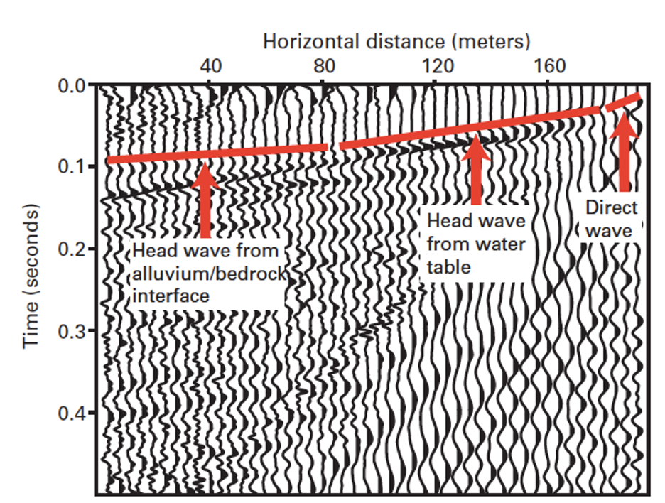
Figure 1. Seismic refraction data showing the interface between the alluvium and bedrock and the top of the water table. Data were collected using a truck-mounted weight-drop as the shot source (Ellefsen, et al., 2007).
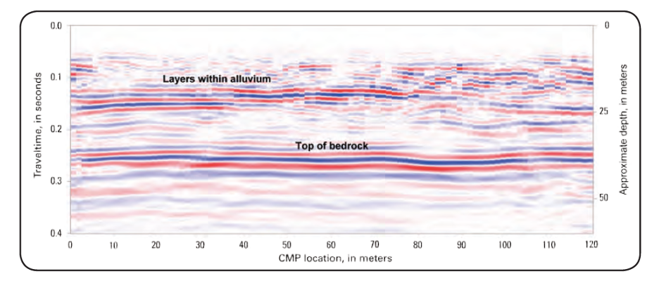
Figure 2. Interpretation of seismic reflection data showing layers of alluvium and the top of bedrock (Lucius, et al., 2007![]() ).
).
Theory of Operation
Seismic refraction and reflection methods employ sound waves to infer subsurface geology. Seismic energy generated by an energy source/shot, such as a hammer strike on a plate, propagates through the ground as seismic compressional waves (P waves) or seismic shear waves (S waves). P waves travel through gases, fluids, and solids, but S waves are transmitted only through materials that have shear strength (i.e., solid material). Seismic refraction methods use time of travel of the first refracted wave to arrive to determine the number, depths, and thickness of subsurface layers. For seismic reflection, travel times and amplitude of the reflected seismic energy are used to define the subsurface structures (Anderson et al., 2008; Benson, et al., 1984). However, using S waves along with P waves in the seismic reflection method may offer higher resolution of thin subsurface features such as clay or sand layers (Johnson and Clark, 1992).
The basis for seismic reflection and refraction is Snell's Law,1 which describes the behavior of sound or light waves across boundaries between layers composed of material with different velocities (Figure 3). As the sound wave moves from one layer to another layer having faster seismic velocities, part of the energy (P wave) is refracted (bent) into the lower layer, and part is reflected (seismic reflection) back into the upper layer. In seismic refraction, if the angle of incidence equals the critical angle, the energy travels along the boundary between the layer with higher velocity (V1) and the layer with lower velocity (V2). As the refracted P wave propagates along the boundary, new P waves are generated and refracted back toward the ground surface (Figure 3). The new P waves are refracted back to the land surface through the first layer at an angle equal to the critical angle (Haeni, 1988).
The amount of energy reflected, refracted, transmitted, or converted depends on the angle of incidence for the P wave and the properties of the two lithologic units (Wightman et al., 2003). Electromechanical transducers (geophones) placed on the ground or in water (hydrophones) sense the return signal from the reflected or refracted waves. In seismic refraction, sound wave travel times are recorded by a seismograph, and in seismic reflection, both travel times and amplitude are recorded. These data are analyzed to determine variations in wave velocities and ultimately interpreted as changes in lithology, fluid saturation, and other geological and hydrogeological information.
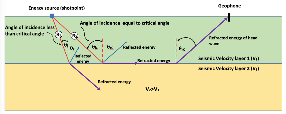
Figure 3. This diagram shows the paths of P waves in the subsurface if seismic velocities in layer 2 are greater than in layer 1 (reflected energy pathways are blue arrows and refracted energy pathways are purple arrows). As P wave R1 moves through layer 1, the angle of incidence is less than the critical angle, so part of the P wave will be refracted into the subsurface, and part of the P wave will be reflected toward the land surface. For P wave R2, the angle of incidence is equal to the critical angle. In this case, part of the energy wave will be refracted to propagate along the upper surface of layer 2. As the refracted energy moves along the boundary between layer 1 and layer 2, new sound waves are created. A portion of the new wave is then refracted back toward the land surface where a geophone can record the travel time (modified from Haeni, 1988).
The fundamental assumptions underlying seismic analysis are:
- Seismic velocities of geologic layers generally increase with depth (for seismic refraction).
- The layers are thick enough to be detected.
- The layers' seismic velocities are varied enough that the individual layers can be identified (Benson et al., 1984).
Ranges of compression wave velocities have been established for various types of soil and rock (Table 2). Because the ranges of velocities for the different materials overlap, determining the unique composition of the layer based on seismic velocities alone is not possible. However, if the seismic data are combined with geologic information such as boring logs, it is possible to identify and correlate lithologic information across a site of investigation (Benson et al., 1984; Wightman et al., 2003).
Table 2. Compression (P) Wave Velocities in Soil and Rock
| Material | Velocity (m/s) |
|---|---|
| Weathered surface material | 305-610 |
| Gravel or dry sand | 465-915 |
| Sand (wet) | 610-1,830 |
| Sandstone | 1,830-3,970 |
| Shale | 2,750-4,270 |
| Chalk | 1,830-3,970 |
| Limestone | 2,140-6,100 |
| Salt | 4,270-5,190 |
| Granite | 4,380-5,800 |
| Metamorphic rocks | 3,050-7,020 |
The velocity at which the P waves travel through the subsurface layers is controlled by the density and elastic properties of the layer. Factors affecting density and elasticity include porosity, mineral composition, and water content. As a general rule, velocities are greater for:
- Dense rocks than light rocks.
- Older rocks than younger rocks.
- Igneous rocks than sedimentary rocks.
- Unfractured rock than fractured rock.
- Unweathered rock than weathered rock.
- Consolidated sediment than unconsolidated sediment.
- Water-saturated unconsolidated sediment than dry unconsolidated sediment.
- Wet soil than dry soil (Benson et al., 1984).
Sites with two- to three-layer systems can be analyzed in the field with simple calculations and nomograms. More complicated sites having three to four layers require computer software to solve the seismic equations. Lateral variations in subsurface materials or irregular boundaries between layers caused by changes in density and/or hardness of the material will create excess noise in the readings. Data analysis is not straightforward; the analyst must be knowledgeable about the method, how the data were collected, and the hydrogeologic conditions of the site (Benson et al., 1984).
Seismic Refraction
For seismic refraction, the layer velocity is calculated from the arrival times of the refracted P waves and the distance of the geophones from the source. The seismic refraction data can be used to estimate the depth of subsurface materials that have different densities and seismic velocities.
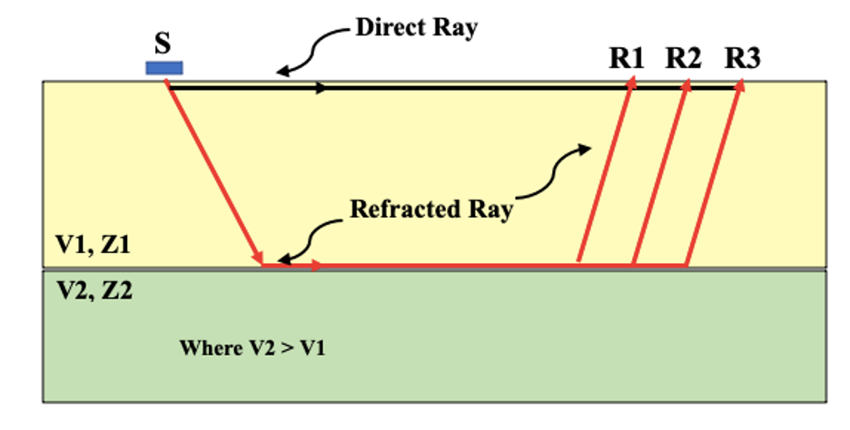
Figure 4. A generalized conception of a seismic refraction configuration (modified from Anderson et al., 2008).
The seismic line or spread consists of an energy source (or shot) location with multiple geophone (or receiver) locations (Figure 4). At each geophone location, the arrival time of the seismic wave is detected. For refraction, the assumption is that velocities increase with depth below land surface so V2 would be greater than V1, and acoustic impedances2 Z2 would be greater than Z1 (Anderson et al., 2008). Seismic refraction measures first arrival refracted waves (called "rays" in Figure 4). At distances longer than the critical distance3 from the source, the refracted waves arrive at the geophone before the direct wave does. Multiple subsurface layers can be detected as long as they are thick enough.
Travel times plotted versus the source-to-geophone distance are used to determine the number of layers in the subsurface, as well as the depths of each layer. The number of layers is indicated by the number of line segments on the plot. The seismic velocity for each layer is the inverse of the slope of the line segment. Depth to the refracting boundary between two layers is calculated by the equation (Benson et al., 1984):
$$ D=\frac{X_c}{2} \sqrt{\frac{\left(V_2-V_1\right)}{\left(V_2+V_1\right)}} $$Where:
D = depth to boundary between Layer 1 and Layer 2
V1 = Velocity of Layer 1 = 1/Slope of the time-distance segment for Layer 1
V2 = Velocity of Layer 2 = 1/Slope of the time-distance segment for Layer 2
Xc = Critical Distance
In general, for seismic refraction, the following should be considered (Benson et al., 1984):
- The method is generally limited to resolving up to five lithologic layers.
- The geologic layers' seismic velocities must increase with depth.
- The layers should be thick enough to be detected.
- The seismic velocities of the layers must be different enough in order to resolve the individual layers.
- The seismic line should be centered over the object/area of interest.
- The overall length or spread of the line should be three to five times the depth of interest.
- The spacing between geophones determines the resolution (closer spacing results in higher resolution).
- The spacing between geophones is commonly 5 to 20 feet, but surveys have been completed with geophone spacings from ½ ft to 50 ft.
Seismic Reflection
For seismic reflection, the amplitude of the P wave is recorded, as well as the arrival times (Wightman et al., 2004):
- Subsurface layers must have different seismic velocities, but layer velocities do not need to increase with depth.
- Seismic reflection can be applied even in low-velocity zones.
- Seismic reflection is best suited for depths of investigation that are greater than 65 feet. Application of reflection to investigations at depths less than 30 feet is complicated by interference of surface waves, direct waves, and refracted waves.
- Geophone spacing within the source-geophone array determines the resolution. For higher resolution of shallow geologic profiles, closer spacing of the geophones may be needed.
- Source-geophone offsets should be at least half of the reflection depth.
- Seismic reflection is one of the more costly geophysical methods, and expertise is required to process the data.
System Components
Both seismic refraction and reflection surveys use a seismic source such as a sledge hammer for depths up to 50 feet; weight drops or small explosive charges are commonly used for target depths up to 100 feet (Wightman et al., 2004). Each hammer strike, weight drop, or small explosive detonation is called a "shot." Multiple subsurface points can be investigated with each shot. Each shot emits seismic energy that propagates out from the source through the subsurface. The seismic signals are recorded on a linear array of geophones (Figure 5) at set distances from the source. The array of geophones is connected to the seismograph, which is connected to a power source (a small battery). The geophones turn the seismic energy (ground motion) into an electrical signal using a velocity transducer or an accelerometer (Wightman et al., 2004). The seismograph records the travel time in milliseconds for each signal received. The amplitude of the signal is also recorded for seismic reflection surveys.
↩Modes of Operation
Seismic data can be collected on the ground surface, in boreholes or cross-boreholes, or from watercraft to evaluate subsurface features below water bodies. These modes are outlined below.
Ground Surface
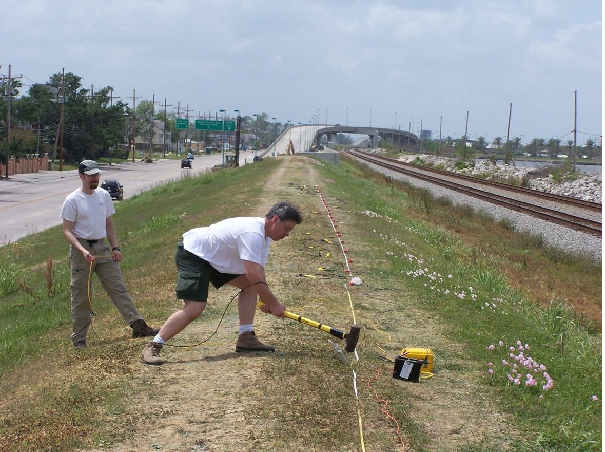
Figure 5. A USGS scientist hits a strike plate with a hammer to initiate a seismic wave in the subsurface. Travel times detected at the red geophones along the survey profile will be recorded by the seismograph (USGS 2006).
For surface applications of seismic investigations, geophones and an energy source are deployed either by hand or from a vehicle. Figure 5 shows a two-person team using a strike plate and hammer as the energy source and a string of geophones (red) to detect the seismic waves generated by the hammer strike. The data are recorded on a seismograph. A hammer is a sufficient energy source for shallow investigations (less than 50 feet).
Light vehicles can also be used to collect seismic data at the ground surface. The rear of the vehicle houses a small weight drop and tows a string of geophones (Figure 6).

Figure 6. USGS hydrologists conduct a seismic imaging survey. The yellow land streamer contains the geophones (red) and is towed behind a vehicle. This relatively new system allows for inexpensive and rapid data acquisition. The survey was conducted as part of an applied research effort by the USGS Office of Groundwater Branch of Geophysics in the Bronx, New York, in 2007 (USGS, 2007).
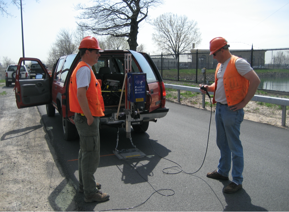
Figure 7. USGS hydrologists prepare equipment for a seismic imaging survey. The accelerated weight-drop energy source (blue box) is attached to the back of the vehicle. The survey was conducted as part of an applied research effort by the USGS Office of Groundwater Branch of Geophysics in the Bronx, New York, in 2007 (USGS, 2007).
For deeper seismic investigations of regional subsurface features, vibration or thumper trucks can be used as the energy source (Figure 8).
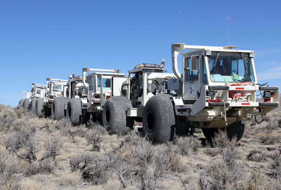
Figure 8. Vibration trucks travel along designated north/south routes applying hydraulic pressure at 160-foot intervals. The seismic waves are then picked up by receiver points within the project area (USGS).
Borehole/Cross-borehole
Seismic methods can also be applied via a single borehole or cross-borehole to evaluate subsurface structures. Figure 9 shows a generalized setup for collecting seismic data from within a single borehole. In cross-borehole applications, sources are deployed down one borehole, and receivers are deployed in another (Figure 10). Multiple sources in the source borehole and multiple geophones in the receiving borehole can be used in cross-borehole applications.
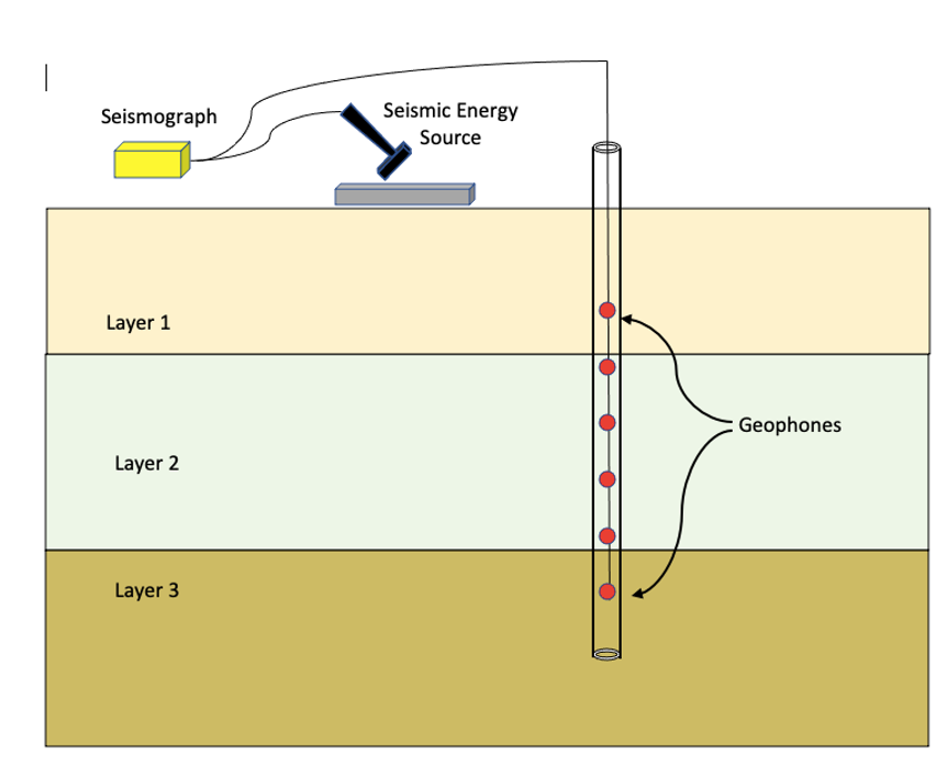
Figure 9. A simplified diagram shows the configuration of geophones, energy source, and seismograph to collect borehole seismic data (modified from Wightman, et al., 2004).
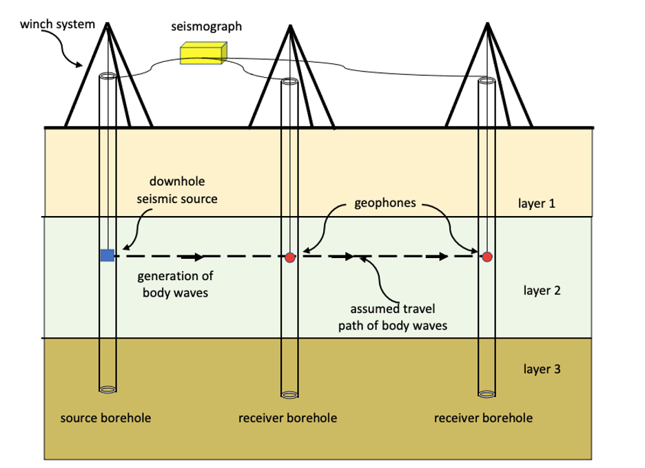
Figure 10. A generalized field setup for the cross-borehole seismic mode. A seismic energy source(s) is deployed in the source borehole with geophone(s) deployed in the receiver borehole (modified from Wightman, et al., 2004).
Watercraft Mode
Seismic data may also be collected beneath water bodies using large or small watercraft. Figure 11 shows a floating sled outfitted with equipment to collect seismic reflection data. This setup can collect seismic data in the subsurface beneath shallow waterbodies.

Figure 11. A USGS scientist stands on a floating sled that enables sub-bottom surveying in shallow water, nearshore, and shore-face environments. The sled is equipped with an EdgeTech SB-512i CHIRP system, and sonar equipment is used to collect sub-bottom seismic reflection data and bathymetry (USGS, 2019).
Figure 12 shows a generalized diagram of a seismic survey vessel towing a string of hydrophones (receivers) along the surface of the water. The seismic energy source on the vessel emits a sound wave that is detected by the hydrophones. Electronic equipment on the vessel records the travel times and amplitude of the waves.
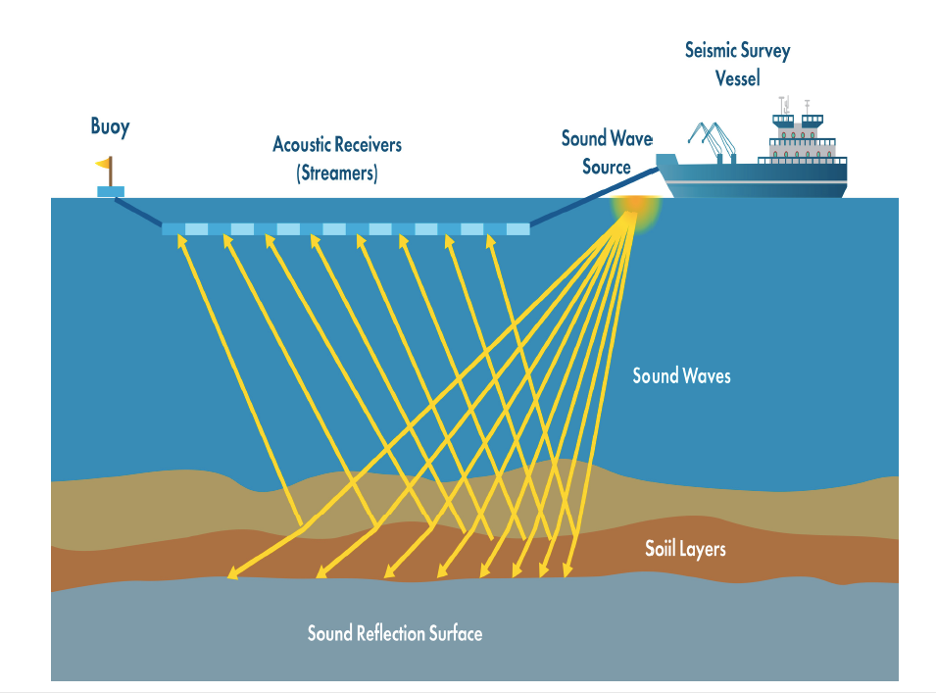
Figure 12. A seismic survey vessel collects seismic data from beneath the subsurface in waterbodies (BOEM, 2018![]() ).
).
Data Display and Interpretation
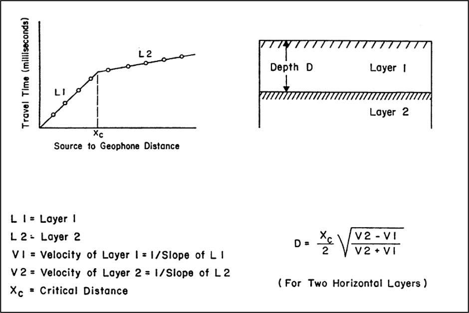
Figure 13. This example travel time-distance plot using one shot and signals from nine geophones depicts the change in slope of the two line segments indicating that two layers were encountered by the P waves. The critical distance xc is found at the breaking point on the plot. If more than two layers were identified, there would be additional xc for each layer encountered, and additional line segments with a change in slope would be evident on the plot. The equation is used in a two-layer system to calculate the depth to Layer 2 (Benson et al., 1984).
Data display and interpretation range from simple time/distance (T/D) plots of raw seismic refraction data to complex 3D models of the subsurface created after pre- and post-processing of the data using special software.
For seismic refraction data, limited interpretation of the raw data is possible in the field:
- Calculations based on the T/D plot can estimate the depth of a lithologic layer.
- The number of line segments will indicate the number of layers encountered (Figure 13).
- The seismic velocity of each responding layer is inversely proportional to the slope of each line segment.
- The critical distance (xc in Figure 13) is identified on the plot by break points in the line. Layer depth can be calculated using critical distance and the velocities (Benson et al., 1984; Baker 1999).
More complex evaluations of the raw data are required to build geologic models of the subsurface. In general, processing seismic data should include the following steps (Baker 1999):
Preprocessing
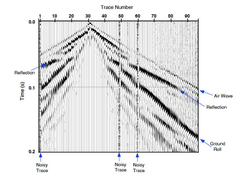
Figure 14. An evaluation of the seismic data in a trace shows some random noise and true reflections (Baker 1999). An "air wave" is noise created by the energy moving through the air rather than the earth. A "ground roll" is noise from a wave traveling along the ground surface (instead of the subsurface).
Seismic data are recorded in one of two standard formats defined by the Society of Exploration Geophysicists: SEG-Y or SEG-2. The two formats differ in the size and format of the trace headers4 and the storage of the trace-amplitude data. The SEG formats must be converted to the format of the specific software package used. To shorten the computational time, the data may be truncated if no reflections are seen below a certain depth. Trace5 locations must be correctly entered into the trace headers so that spatial processes such as velocity calculations will be correct. Data should be evaluated to look for true reflections versus noise such as air waves (created by the energy moving through the air rather than the earth) or ground roll (created by a wave traveling along the top of the ground surface rather than through the subsurface [Figure 14]). True reflections should be identifiable on several records with little processing and should remain visible over a range of frequencies (Baker 1999).
Improving Signal to Noise Ratio (S/N)
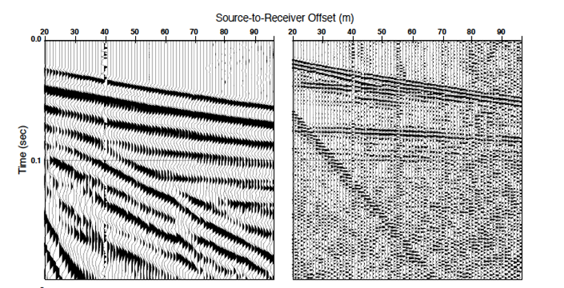
Figure 15. Unfiltered shot gathers on the left compared to frequency filtered shot gathers on the right. Low-frequency noise has been removed by the filter (Baker, 1999).
There are three ways to improve S/N in seismic data: 1) attenuating noise through filtering; 2) correcting for spatial/temporal shifts in traces; and 3) stacking. Noise can be attenuated by muting if it has a unique travel time or by filtering for frequency-wave number if the noise has a unique frequency from the reflections (Figure 15). If conditions in the subsurface do not meet the layered-earth assumption, there can be spatial shifts in the data. Because the time of travel for P waves is correlated to the distance between shot and receiver and velocity of P waves, heterogeneities in lateral velocities may distort travel times and appear as false structures in the seismic data. Differences in source and receiver elevations can also cause temporal shifts. Stacking of the data can resolve some noise issues. In stacking, multiple traces from different shot records with a common reflection point are combined into a single trace. The stacking process increases the reflection signal in amplitude, making it easier to discriminate between noise and reflections.
Stacking and Verification
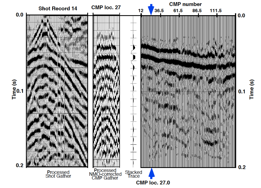
Figure 16. Figure 16. A comparison of the stacked trace and the original shot gathers validates the post-processing result (Baker, 1999).
Not only is stacking of the seismic data part of the velocity analysis process, it is also a critical final step before interpretation of the data. Reflections observed on the stacked section should be corroborated by comparing the stacked section to the original shot gathers, processed shot gathers, CMP gathers6, and NMO-corrected7 gathers (Figure 16) (Baker, 1999).
Data Display
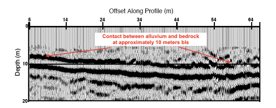
Figure 17. An example of a depth section showing the interface between the Paleozoic bedrock and Holocene fluvial deposits at approximately 10 meters below land surface (Baker, 1999).
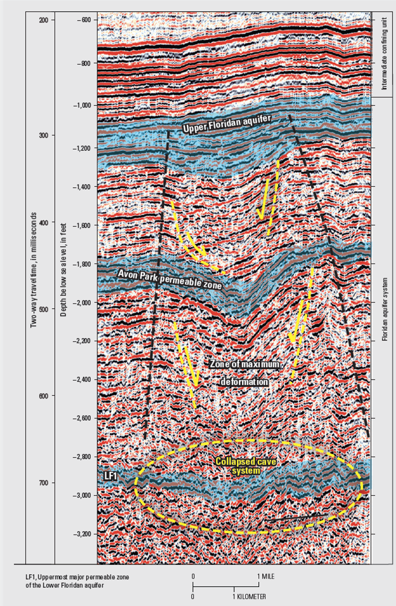
Figure 18. An example of seismic reflection data used to interpret geologic structures in the subsurface. The blue highlighted zone represents more permeable zones. The yellow dashed lines represent possible major faults cutting across confining units that may provide a pathway for vertical migration of groundwater between permeable zones (Cunningham, 2013).
Determining the depth to a geologic unit or formation in the subsurface is usually a goal of collecting seismic data. This is done by converting seismic time sections to depth sections using the velocity function calculated as part of the velocity analysis. Stacked velocities are converted to velocities of the lithologic layers using the Dix equation8. Using the layer-specific velocities, depth sections are created by mapping the travel time data (Figure 17). Other data such as borehole data, refraction, or outcrop data can be used to ground truth the depth section (Baker, 1999).
For complex subsurface structures where there are steeply dipping beds or significant heterogeneities, a person with a significant understanding of the principles of seismic reflection and refraction should analyze the data. If borehole information is available, a person with experience and expertise can create an interpretation or model of the geologic structures in the subsurface (Figure 18). For example, seismic depth sections can show buried stream channels or fracture zones in bedrock that would indicate a zone of potential contaminant migration (Anderson et al., 2008; Baker 1999).
↩Performance Specifications
The performance specifications (Table 3) for seismic reflection and refraction used at groundwater sites include the shot (or energy source), length of seismic line, shot to receiver offset, geophone spacing, spacing between the shots, the seismograph, vertical resolution, and lateral resolution.
Table 3. Seismic Methods Specifications
| Attribute | Description |
|---|---|
| Shot (energy source) | For near-surface targets, hammer blows or weight drops are used, as well as small explosive charges. The energy source can influence the width of the frequency spectra. A hammer can be used for obtaining data depths of less than 30-50 feet. For depths of 100 feet or greater, a 500-pound drop weight is needed. In areas with excessive noise, a more powerful energy source may be needed. |
| Length of seismic line (spread) | The total survey line length consisting of multiple geophones should be three to five times the depth of interest. The quality of the velocity analysis and reflection depth determination is influenced by the spread length. |
| Shot to receiver offset | This offset is the distance between the shot and the center of a group of geophones in a seismic line. A general guideline for seismic reflection surveys is that the shot to receiver offset should be at least half of the anticipated reflection depth. |
| Geophone spacing | The geophone spacing ∆xG, should adhere to the following criterion ∆xG <λmin/2=vmin *Tmin, where λmin is the smallest wavelength, vmin is the propagation velocity, and Tmin is the signal period. Geophone spacing of 10 to 50 feet is common, but closer spacing is used for higher resolution. |
| Spacing between shots | If significant lateral heterogeneities in seismic velocity are expected in the upper layer, the shot (energy source) spacing should not exceed the distance at which the direct wave can be detected. |
| Seismograph | The seismograph records the measurements detected at the geophones. Seismographs come as single-channel units or multi-channel units. Multi-channel units increase the rate of data collected. Multiple geophone signals can be recorded simultaneously using the multi-channel units. This allows for more control over filtering of signals to remove noise. |
| Vertical resolution | In typical environmental applications, lithologic layers with thicknesses of three to 30 feet can be resolved. |
| Lateral resolution | In typical environmental applications, lateral resolution is significantly less than vertical resolution. Higher frequencies and shallower depths allow for better lateral resolution. Lateral resolution decreases with depth. |
Benson et al., 1984; Rabbel, 2009, SEG Wiki, 2014 and 2018
↩Advantages
Seismic refraction is a relatively simple and adaptable method for shallow subsurface investigations. While seismic reflection and seismic tomography surveys may require more equipment, personnel, and data processing, they can provide greater detail of subsurface conditions. The following advantages of seismic methods were adapted from Anderson and Ismail 2006![]() and EPA 1993
and EPA 1993![]() :
:
Table 4. Advantages to Using Seismic Methods For Site Characterizations
| Method | Advantages |
|---|---|
| Seismic Refraction |
|
| Seismic Reflection |
|
| Seismic Tomography |
|
Limitations
While seismic methods are a useful tool in site characterization, their application may be limited by subsurface conditions, availability of personnel, and costs. The following limitations of seismic methods were adapted from Anderson and Ismail 2006| Method | Limitations |
|---|---|
| Seismic Refraction |
|
| Seismic Reflection |
|
Cost
The current average equipment rental rate is approximately $700/week for a 24-channel seismic recorder with a set of geophones and cables. Costs for a completed seismic survey (data collection, analysis, and interpretation) range from $1,000-$2,000 per day for a seismic refraction survey to $2,000-$4,000 per day for a seismic reflection survey (ITRC, 2019).
↩Case Studies
Environmental Impact Assessment of the Subsurface in a Former W-SN Mine: Integration of Geophysical Methodologies
De Almeida, H., M.C.G. Marques, H. Sant'Ovaia, R. Moura, and J. Espinha Marques, Minerals 13(1):55(2023)
This research proposes an innovative approach that integrates different geophysical techniques to characterize the impact of mining activity on the subsurface in an area surrounding the tungsten mine of Regoufe in northern Poland. Sulfide-rich tailing accumulation may have caused acid mine drainage (AMD), where leaching led to soil contamination, as evidenced by its acidic character and anomalous concentrations of Potentially Toxic Elements (PTE). Electrical resistivity and electromagnetic geophysical methods were used to measure subsurface electrical properties. In addition, seismic refraction and multichannel analysis of surface waves were performed to characterize the geometry, depth, and geomechanical behavior of the soil and rock bodies. Integrating these techniques allowed the interpretation of hydrogeological sections and a 3D resistivity volume to gain insight into the distribution of potentially contaminating fluids and tailings material present in the mining valley.
Environmental Investigation Using Geophysical Data at East Sadat City, Egypt
Araffa, A., et al., Egyptian Journal of Petroleum, Vol. 28, Issue 1, March 2019
Resistivity, seismic refraction, and ground penetrating radar (GPR) were applied to delineate the depth to the groundwater surface, subsurface stratigraphy, and subsurface structures that control the configuration and distribution of the groundwater aquifer.
Integrating Seismic-Reflection and Sequence-Stratigraphic Methods to Characterize the Hydrogeology of the Floridan Aquifer System in Southeast Florida
Cunningham, K., U.S. Geological Survey Open-File Report 2013-1181, August 2013
Seismic reflection and borehole data were integrated into an improved geologic and hydrogeologic framework to provide a better understanding of the structural and stratigraphic features that influence groundwater flow and contaminant transport in the Floridan aquifer system.
Seismic Reflection and Refraction Study of a Landfill
De Iaco, R., et al., Journal of Applied Geophysics, Vol. 52, Issue 4, March 2003
A high-resolution seismic profile was recorded in an attempt to delineate the base of a landfill and map the geometries of the host sediments. Although independent applications of the seismic reflection and refraction techniques were not successful in meeting the survey objectives, a combination of the two approaches constrained by borehole information provided the required details on the landfill and surrounding sediments. This study highlights the limitations of employing 2-D seismic refraction and reflection methods for resolving problems in highly heterogeneous 3-D media.
Integrated Use of Continuous Seismic-Reflection Profiling and Ground-Penetrating Radar Methods at John's Pond, Cape Cod, Massachusetts
Powers, C. and F. Haeni, Symposium on the Application of Geophysics to Engineering and Environmental Problems, Oakland, California, March 14-18, 1999, Proceedings: Wheat Ridge, Colo., Environmental and Engineering Geophysical Society, p. 359-368
The U.S. Geological Survey conducted continuous seismic-reflection profiling and ground penetrating radar surveys in April 1998 over the northern part of a glacial kettle pond southeast of Otis Air National Guard Base, Cape Cod, Massachusetts. The surveys were conducted to delineate the types and thickness of sedimentary units that may control the infiltration of contaminated groundwater into the pond. The two methods provided complementary information over most of the surveyed part of the pond. The data were interpreted to generate a bathymetric map and a map of sediment type and thickness beneath John's Pond.
Use of Geophysical Profiling to Guide Groundwater Remediation Studies
Watson, D., et al., Environmental Sciences Division, Oak Ridge National Laboratory, Technical Report. No date.
Multi-electrode resistivity methods and pseudo-tomographic seismic refraction techniques were used to image to a depth of approximately 30 m at the Natural and Accelerated Bioremediation Research Field Research Center, a research site that has been developed by the U. S. Department of Energy to study bioremediation methods. The site is known to contain nitrates, uranium, and other contaminants. These geophysical methods were effective in delineating the plume and in defining geologic units that appear to influence contaminant transport. Extensive drilling and groundwater sampling verified the geophysical data.
↩References:
Anderson, N., et al., 2008. ![]() Geophysical Methods Commonly Employed for Geotechnical Site Characterization. Transportation Research Circular E-C130, pp. 44, October.
Geophysical Methods Commonly Employed for Geotechnical Site Characterization. Transportation Research Circular E-C130, pp. 44, October.
Anderson, N. and A. Ismail, 2006. ![]() A Generalized Protocol for Selecting Appropriate Geophysical Techniques.
A Generalized Protocol for Selecting Appropriate Geophysical Techniques.
Baker, G., 1999. Processing Near-Surface Seismic-Reflection Data: A Primer. Course Notes Series, No. 9, Society of Exploration Geophysicists.
Benson, R., 2006. Remote Sensing and Geophysical Methods for Evaluation of Subsurface Conditions. In: David M. Nielsen (editor), Practical Handbook of Ground Water Monitoring. Lewis Publishers, Inc. Chelsea, Michigan. pp.249-296.
Benson, R., R.A. Glaccum, and M.R. Noel, 1984. Geophysical Techniques for Sensing Buried Wastes and Waste Migration. EPA-600/7-84-064, pp. 256, June.
Bureau of Ocean and Energy Management, 2018. ![]() Geological and Geophysical Surveys. November.
Geological and Geophysical Surveys. November.
Cunningham, K., 2013. Integrating Seismic-Reflection and Sequence-Stratigraphic Methods to Characterize the Hydrogeology of the Floridan Aquifer System in Southeast Florida. U.S. Geological Survey Open-File Report 2013-1181, pp. 8.
Day-Lewis, F.D., C.D. Johnson, L.D. Slater, J.L. Robinson, J.H. Williams, C.L. Boyden, D. Werkema, and J.W. Lane, Jr., 2016. A Fractured Rock Geophysical Toolbox Method Selection Tool: Groundwater.
Ellefson, K., B. Burton, J. Lucius, S. Haines, D. Fitterman, J. Witty, D. Carlson, B. Milburn, and W. Langer, 2007. Field Demonstrations of Five Geophysical Methods That Could Be Used to Characterize Deposits of Alluvial Aggregate. U.S. Geological Survey Scientific Investigations Report 2007-5226, pp. 20.
Ellefson, K., J.E. Kibler, P.A.Hsieh, and A.M. Shapiro, 1998. Crosswell Seismic Tomography at the USGS Fractured Rock Research Site Data Collection, Data Processing and Tomograms. Open-File-Report 980510.
Everett, Mark E., 2013, Near-surface applied geophysics. Cambridge University Press.
Haeni, F., 1988. Application of Seismic-Refraction Techniques to Hydrologic Studies. Techniques of Water-Resources Investigations of the United States Geological Survey, Chapter D2, pp. 95.
ITRC (Interstate Technology & Regulatory Council), 2019. Implementing Advanced Site Characterization Tools. ASCT-1. Washington, D.C., Advanced Site Characterization Tools Team
Johnson, W. and J. Clark, 1992. Improving Subsurface Resolution With the Seismic Reflection Method: Use S-Waves. Ground Water Management 11: 655-663 p.
Kirsch, R., 2009. Groundwater Geophysics, A Tool for Hydrogeology. Chapter 1, pp. 556.
Lucius, J., et al., 2007. ![]() An Introduction to Using Surface Geophysics to Characterize Sand and Gravel Deposits. U. S. Geological Survey Circular 1310, pp. 33.
An Introduction to Using Surface Geophysics to Characterize Sand and Gravel Deposits. U. S. Geological Survey Circular 1310, pp. 33.
Rabbel, W., 2009. Groundwater Geophysics, A Tool for Hydrogeology. Chapter 2, pp. 556.
SEG Wiki, 2014. SEG Wiki Dictionary. Webpage consulted August 2022.
SEG Wiki, 2018. SEG Wiki Dictionary. Webpage consulted June 2022.
Schlumberger, 2022. Schlumberger Oilfield Glossary. Webpage consulted August 2022.
U.S. EPA, 1993. ![]() Use of Airborne, Surface and Borehole Geophysical Techniques at Contaminated Sites: A Reference Guide. EPA/625/R-92/007, pp. 304. September.
Use of Airborne, Surface and Borehole Geophysical Techniques at Contaminated Sites: A Reference Guide. EPA/625/R-92/007, pp. 304. September.
Wightman, W.E. et al., 2004. Application of Geophysical Methods to Highway Related Problems. Federal Highway Administration, FHWA-IF-04-021, pp. 744, September.
Yilmaz, Ö., 2001. Seismic Data Analysis. Investigations in Geophysics, Volume 1, Society of Exploration Geophysicists.
Helpful Information
-
$$ \frac{\sin i}{V_1}=\frac{\sin r}{V_2} $$ where i is the angle of incidence and r is the angle of refraction. V1 is the velocity in the upper medium, and V2 is the velocity of the underlying medium. ↩
-
$$ \frac{\sin i}{V_1}=\frac{\sin r}{V_2} $$ where i is the angle of incidence and r is the angle of refraction. V1 is the velocity in the upper medium, and V2 is the velocity of the underlying medium. ↩
-
Acoustic impedance is a physical property of a material. It is the product of the material's density and seismic velocity (Wightman et al., 2003). ↩
-
Acoustic impedance is a physical property of a material. It is the product of the material's density and seismic velocity (Wightman et al., 2003). ↩
-
In seismic refraction methods, the critical distance is defined as the distance beyond which the refracted wave will reach the geophone before the direct wave. While the refracted wave path is longer than the direct wave path, a portion of the refracted wave path occurs within the higher-velocity layer in the lower geologic unit. At critical distance, enough of the wave travels through the higher-velocity layer to enable the refracted wave to reach the geophone before the direct wave does (Benson, R., et al., 1984). ↩
Trace headers contain information about the data contained in the trace, such as shot point number, trace number, and offset (horizontal distance between source and receiver). ↩
Trace headers contain information about the data contained in the trace, such as shot point number, trace number, and offset (horizontal distance between source and receiver). ↩
A trace is the seismic data collected on one channel of a seismograph. It represents the response of the energy wave to velocity and density contrasts between the rock and sediment layers/interfaces as the wave travels from the shot (energy source) through the subsurface to the receivers (Schlumberger, 2022). ↩
A trace is the seismic data collected on one channel of a seismograph. It represents the response of the energy wave to velocity and density contrasts between the rock and sediment layers/interfaces as the wave travels from the shot (energy source) through the subsurface to the receivers (Schlumberger, 2022). ↩
Individual seismic traces are assigned to the midpoint between the shot and receiver location for that trace. Common Midpoint (CMP) gathers are composed of individual traces with the same midpoint location (Baker, 1999). ↩
- Individual seismic traces are assigned to the midpoint between the shot and receiver location for that trace. Common Midpoint (CMP) gathers are composed of individual traces with the same midpoint location (Baker, 1999). ↩
Normal moveout (NMO) is defined as recorded travel time for a reflection of a source-receiver pair separated by some distance minus the travel time of a "normal" or completely vertical sounding (Baker, 1999). ↩
Normal moveout (NMO) is defined as recorded travel time for a reflection of a source-receiver pair separated by some distance minus the travel time of a "normal" or completely vertical sounding (Baker, 1999). ↩
Dix equation is used to calculate an interval velocity between a series of flat parallel layers.
Vint = [(t2 VRMS22 - t1 VRMS12) / (t2 - t1)]1/2,
where
Vint = interval velocity
t1 = travel time to the first reflector
t2 = travel time to the second reflector
VRMS1 = root-mean-square velocity to the first reflector
VRMS2 = root-mean-square velocity to the second reflector (Schlumberger) ↩Dix equation is used to calculate an interval velocity between a series of flat parallel layers.
Vint = [(t2 VRMS22 - t1 VRMS12) / (t2 - t1)]1/2,
where
Vint = interval velocity
t1 = travel time to the first reflector
t2 = travel time to the second reflector
VRMS1 = root-mean-square velocity to the first reflector
VRMS2 = root-mean-square velocity to the second reflector (Schlumberger) ↩