
Geophysical Methods
Magnetometry
A magnetometer is a tool used for locating ferromagnetic materials (iron, nickel, cobalt, and their alloys) in the subsurface (Table 1). Non-ferromagnetic metals will not be detected by a magnetometer. Magnetometers can detect the ambient magnetic fields emanating from natural ferromagnetic minerals or buried materials such as wells, drums, tanks, pipelines, and debris that could be sources of contamination or components in a conceptual site model (CSM). Magnetic fields are imperceptible to human senses and are similar to lines of force or flux that continuously loop around a magnet from one pole to another. Locating ferromagnetic materials depends on the magnetic susceptibility of the object. The intensity of magnetic flux is related to the magnetic susceptibility of an object. In other words, the greater the magnetic susceptibility of an object, the greater the magnetic flux.
Table 1. Ferromagnetic and Non-Ferromagnetic Metals
| Ferromagnetic Metals | Non-Ferromagnetic Metals |
| Iron | Aluminum |
| Iron Alloys | Copper |
| Steel | Brass |
| Cobalt | Stainless Steel |
| Nickel | Titanium |
Magnetometers should not be confused with metal detectors, which can detect non-ferromagnetic metals, such as aluminum, brass, copper, titanium, and both non-magnetic (non-ferrous) and magnetic (ferrous) stainless steel, as well as ferromagnetic metals.
Typical Uses
A magnetometry survey can help refine the CSM in many ways. For instance, it can:
- Identify buried ferromagnetic tanks, drums or fragments of drums, pipes, and other sources of soil and groundwater contamination.
- Locate abandoned wells, if wells have a ferromagnetic casing or well cover.
- Define the lateral extent of landfills and trenches if the buried waste includes ferromagnetic materials.
- Locate potential ferromagnetic obstacles (like utility hole covers, valve boxes, and piping) in areas of proposed excavation, to avoid damaging buried utility structures or identify items that may pose a hazard during excavation.
- Locate steel-reinforced foundations of buildings below grade.
- Define lateral extent of buried ferromagnetic slag.
- Differentiate and segregate ferromagnetic from non-ferromagnetic metal masses by comparing electromagnetic data to magnetic data.
- At shallow depths, differentiate between large and small ferromagnetic masses based on the strength of the signal detected by the magnetometer. Large masses will have a stronger signal while small masses will have a weaker signal.
- Locate and define extent of buried ferromagnetic ordnance and shrapnel debris.
Magnetometry data can help identify contaminant sources, contaminated media, and potential exposure pathways to refine the CSM, leading to a more effective remedial strategy. For example, locating and removing leaking buried drums will eliminate a continuing source of contamination prior to remediating soil and groundwater. Since fluid flow in the near subsurface often follows the path of least resistance, utility trenches commonly provide high permeability and high-porosity zones which magnetometry surveys and electromagnetic surveys successfully identify. Identifying subsurface utilities with magnetic or electromagnetic surveys can help identify potential transport pathways.
↩Theory of Operation
General Theory
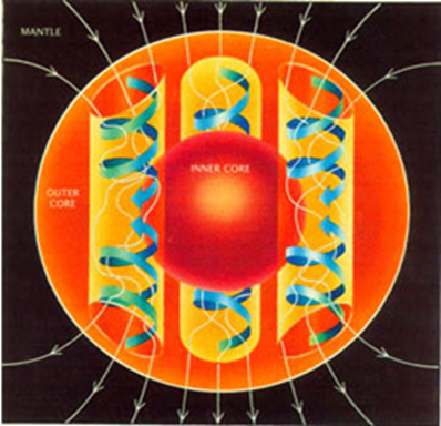
Figure 1. The Earth's outer core acts like an electrical generator converting convective kinetic energy into electrical and magnetic energy. This process is a result of the radioactive heating and chemical differentiation that occurs in the Earth's outer core (USGS).
Objects that generate magnetic fields, including the Earth (Figure 1), are analogous to a bar magnet (Benson et al., 1984) having positive and negative ends that attract and repel within their area of influence. Magnetic lines of force, or flux, are strongest at the ends of a magnet or dipole. The Earth, for example, has its strongest flux at the North and South Poles and a weaker flux near the equator (Figure 2). The same principle applies to a bar magnet, or any ferromagnetic object resembling a dipole configuration such as a pipe or drum. The magnetic field of an object depends on its orientation, shape, condition1, and other factors (Benson et al., 1984).
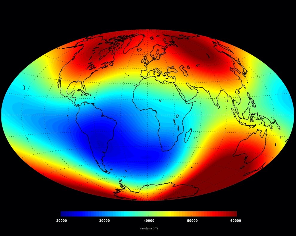
Figure 2. The average strength of the Earth's magnetic field at the surface (in nanotesla). The intensity of the magnetic field is greatest at the poles (NASA).
A steel drum, for example, can be approximated by a magnetic dipole and will have its own variations of magnetic lines of force. The magnetic susceptibility from a drum made of ferromagnetic material will attract the Earth's magnetic field, increasing the magnetic flux near the drum. This change is known as an "anomaly," and it is measured by the magnetometer. The amount of measurable change will vary due to the amount and condition2 of magnetic mass present and its distance from the measuring point of the magnetometer.
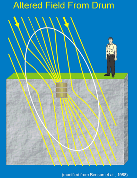
Figure 3. An example of a local anomaly created by a buried steel drum (Benson et al., 1988).
The two most common magnetometers used in environmental investigations are:
- Proton Precession Magnetometer3 (Conventional Free Precession and Overhauser; see Figure 4a).
- Optically Pumped Magnetometer4 (see Figure 4b).
These methods specifically measure the intensity of the Earth's magnetic field vector independent of its direction. When proton precession magnetometers and optically pumped magnetometers are configured with a single sensor, they measure the Earth's total intensity of the magnetic field at the sampling location. They are not sensitive to orientation of the sensor (Benson et al., 1984![]() ). Dual sensor configurations of these magnetometers allows for gradient measurements of the magnetic field intensity which removes the regional magnetic field.
). Dual sensor configurations of these magnetometers allows for gradient measurements of the magnetic field intensity which removes the regional magnetic field.
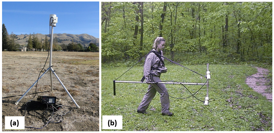
Figure 4. Examples of magnetometers used in magnetic ground surveys: (a) a proton precession magnetometer. (Geomatrix Earth Science LTD used with permission) and (b) an optically pumped magnetometer (J. Ursic, EPA Region 5).
Although these two magnetometers measure magnetic field intensity, the principles used to obtain a measurement are different. The basic differences between the two types of magnetometers are their measurement efficiencies, which can be categorized as either instrument accuracy or data acquisition cycle rate (Table 2). Instrument accuracy is usually measured in nanoteslas5 (nT), the official International System (SI) unit, although gamma (γ) also is used. Magnetometers capable of measuring the smallest changes in nT or γ are more sensitive instruments that can detect smaller or deeply buried masses. Data acquisition cycle rates are typically measured in seconds. Faster acquisition cycle times increase the data collection rate and, thus, reduce time in the field.
Table 2. A Comparison of Proton Precession Magnetometers to Optically Pumped Magnetometers
| Method | Accuracy | Data Acquisition Cycle Rates | Advantages | Disadvantages |
| Proton Precession: Conventional-Free6 | Conventional-Free: 0.1nT | Conventional: 3 to 5 seconds |
|
|
| Proton Precession: Overhauser7 | Overhauser: 0.2nT | Overhauser: 0.5 to 3 seconds |
|
|
| Optically Pumped8 | 0.01nT | 0.1 second |
|
|
OpenEI; Ernstson, 2009; Indian Institute of Geomagnetism
↩System Components
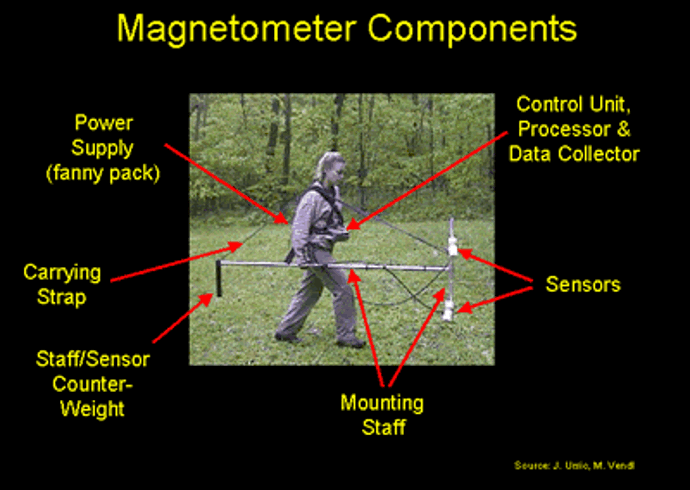
Figure 5. System components for a magnetometer (J. Ursic, EPA Region 5).
Most magnetometers have one or two sensors on a collapsible aluminum mounting staff, a power supply (with external charger), and a control unit with processor. Most magnetometers have built-in data acquisition systems that are part of the control unit and processor (see Figure 5). Systems are self-contained and can be carried and operated by one person using a back or waist pack (Benson et al., 1984).
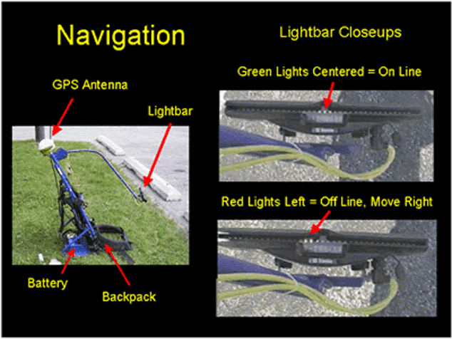
Figure 6. Optional navigation components including GPS eliminate the need for surveying the grid or transect prior to collecting the magnetic data (J. Ursic, EPA Region 5).
Optional support equipment includes an external serial connection port for a global positioning system (GPS) and parallel swathing guidance systems linked to a GPS (Figure 6). This option eliminates the need for pre-surveying a grid, provided the GPS antenna has an unobstructed view of the sky. Although most magnetometer systems include software for processing data, typically more sophisticated programming software is used to interpret data.
All systems operate using onboard battery systems with battery life ranging from four to 12 hours depending on the type of magnetometer and how it is configured (one or two sensors). Most units have rechargeable battery packs.
Specialized System Components
Some geophysical service companies have configured multiple off-the-shelf magnetometers with specialized data collection systems and towing equipment to acquire data for specific purposes. For example, connecting several magnetometers together in a line perpendicular to the direction traversed by a towing vehicle can collect data over a large swath to detect unexploded ordnance.
Marine magnetometers are similar to land-based systems but use a special housing that can be towed underwater behind a boat in navigable waterways. Airborne systems are also available, but are practical only for large-scale uses (i.e., measured in miles).
Optional support equipment, such as GPS, can be rented or purchased from the manufacturer. More accurate and sensitive detector systems typically are more expensive. Vendor services that provide equipment and operators usually have fixed prices, per day or per week, for conducting magnetometer surveys.
↩Modes of Operation
Magnetometers can be configured and operated to eliminate most unwanted atmospheric or solar disturbances that can interfere with locating ferromagnetic objects when using proton precession and optically pumped systems. Magnetometers can be small, handheld instruments that the operator uses by walking a traverse or grid of measurement locations. Magnetometers can also be deployed via watercraft, aircraft, or motor vehicle (Benson et al., 1984; EPA 1993). This section focuses on the handheld method of data collection.
There are three modes of operation for handheld magnetometers categorized by how the sensors are configured (Table 3).
Table 3. Modes of Magnetometer Operation
| Mode | Sensor Configuration | Advantages | Disadvantages |
| Total Field | One Mobile Sensor | Detection limits are slightly deeper than gradient mode. | Cannot correct for atmospheric disturbances. |
| Requires only one sensor, and the equipment is less expensive to purchase or rent. | Erroneous data can unknowingly be collected. | ||
| Total Field with Base Station | One Mobile Sensor and One Static Base Station Sensor | Multiple mobile total field sensors can be used with one base station. | Base station must be established in a secure area and protected from nearby external ferromagnetic fields (e.g., passing cars). |
| Detection limits are slightly deeper than gradient mode. | Data from total field sensor(s) and base station must be merged prior to interpretation to statistically correct for atmospheric disturbances. | ||
| Gradient | Two Attached Mobile Sensors (gradiometer) | Automatic correction for atmospheric disturbances. | Detection limits are slightly shallower than total field mode. |
| Both sensors can be carried by operator, and no base station needed. | More expensive to purchase than total field systems. |
Generally, in all modes and configurations, sensors are placed at the end of horizontal or vertical poles (depending on design or operator needs) held away from the operator to reduce effects from small amounts of ferromagnetic metal that typically cannot be removed (e.g., eyeglasses and steel toe boots). Sensors can also be mounted high off the ground to eliminate interference from surface debris or close to the ground to obtain measurements from a very minor or small mass.
↩Total Field Mode
Figure 7. If a single sensor is used, the total magnetic field at that location is measured. Magnetic data collected using this method include the response of the anomaly and the fluctuations in atmospheric magnetic data. Data are not corrected for atmospheric disturbances (Geomatrix Earth Science LTD used with permission).
The total field mode uses one sensor to measure the strength of a magnetic field (Figure 7). Data consist of one measurement (in gammas or nanoteslas). This mode is rarely used at environmental remediation sites in isolation since it is susceptible to atmospheric disturbances, such as intense solar activity, which could mask small anomalies.
↩Total Field with Base Station Mode
This mode counteracts and minimizes the effect of solar or atmospheric activity on the magnetometer. One stationary base station collects reference data while one or more total field sensors move around. Both are programmed to automatically collect data at short intervals that range from several seconds to several minutes. After all data are collected by the operator(s), each system is connected to the base station for an automatic data merge. Built-in programs use a statistical method to segregate the base station data and operator system data into segments with data collected at or near the same moment in time. After segments are segregated, the base station data are individually subtracted from the operators' mobile station data. This resulting positive or negative value is the best statistical determination for correcting unwanted atmospheric changes. The data are expressed in corrected gammas or corrected nanoteslas.
Gradient Mode
The gradient mode also counteracts and minimizes the effect of solar or atmospheric activity. In the gradient mode, the magnetometer (also known as a "gradiometer" in this mode) sensors can be configured vertically or horizontally. In the vertical configuration, the operator carries two mobile sensors (Figure 5) separated by a vertical distance of usually one-half or one-meter perpendicular to the ground (for upper northern and southern latitudes). Typically, after data are collected, a built-in program subtracts the lower sensor data from the upper sensor. The resulting positive or negative value provides a gradient reading. Regional trends and fluctuations in the Earth's magnetic field are removed by using a gradiometer (Benson, et al., 1984![]() ). The data are expressed in gammas or nanoteslas per meter (γ/m or nT/m).
). The data are expressed in gammas or nanoteslas per meter (γ/m or nT/m).
Anomalies from shallow sources are enhanced in gradient measurements in the vertical configuration. However, enhanced surface signals can obscure the target anomalies. Table 4 shows the advantages and disadvantages of using either the vertical or horizontal sensor configuration of the gradient mode.
Table 4. Gradient Mode Sensor Advantages and Disadvantages
| Sensor Configuration | Advantages | Disadvantages |
| Vertical | Good depth resolution. Enhances shallow features. | Less detail for linear objects. |
| Horizontal | Good delineation for linear objects, such as pipelines. | Less detail for deeper features. |
Survey Design
In designing a magnetic survey, several factors should be considered:
- Composition of the target object – Lower ferromagnetic content means decreased distance at which the object can be detected.
- Size and mass of the object – Objects that are large or have a large mass will generally have stronger magnetic fields that emanate much farther than small masses. As a result, a larger survey grid may be used for locating larger masses, while a smaller survey grid is required for smaller masses.
- Depth of the object – In general, smaller objects emit weaker magnetic fields that may be detectable only when the objects are near the surface. However, if multiple objects are grouped together or stacked on top of one another, they will emit a stronger magnetic field that can be detected at greater depths.
- Physical surroundings – If the material surrounding a ferromagnetic object also contains ferromagnetic materials, it may mask the magnetic field emanating from the object. For example, a drum buried in soil containing ferromagnetic ores or slag will be difficult to detect. Nearby buildings, vehicles, power lines, and fences may also interfere with detection.
- Orientation and condition of the object(s) – Ferromagnetic objects have stronger and weaker magnetic fields emanating through the mass that follow the geometry of the object. The stronger fields are usually near the ends of the mass. Magnetic fields are weaker if the object's shape is distorted. For example, a crushed drum has a weaker magnetic signal than an intact drum.
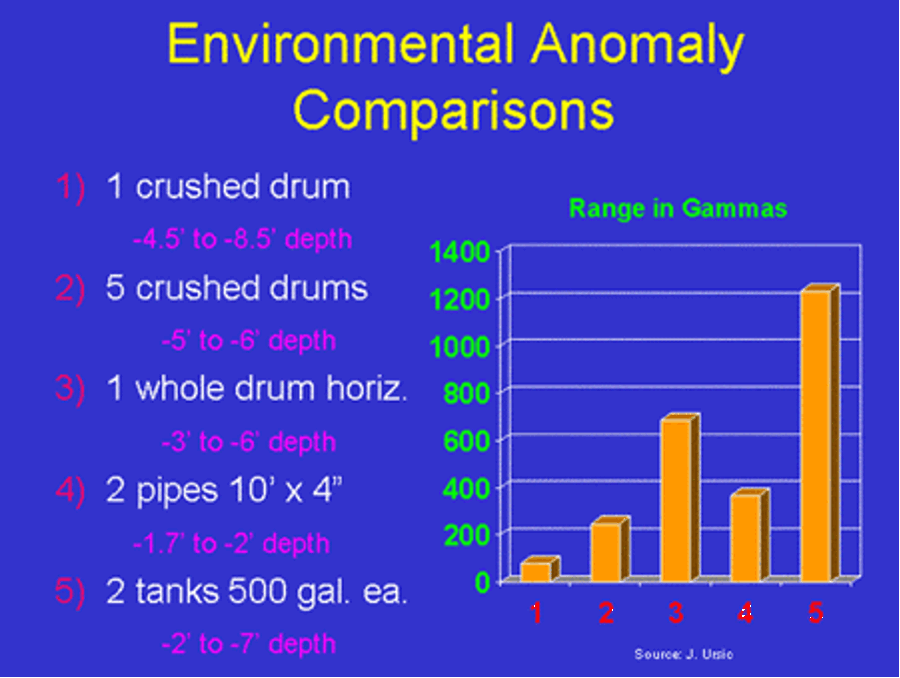
Figure 8. Intact objects have stronger magnetic signals than distorted objects, and larger objects have stronger signals than smaller objects (J. Ursic, EPA Region 5).
In general, the depth of the investigation is limited by the mass and magnetic susceptibility of the object(s) being observed. As a general rule, the larger the mass of an object, the deeper the depth of an investigation that can be achieved. As shown in Figure 8, a 500-gallon tank will have a much stronger signal (1200γ or nT) as compared to the signal of a single 55-gallon drum (approximately 700γ or nT).
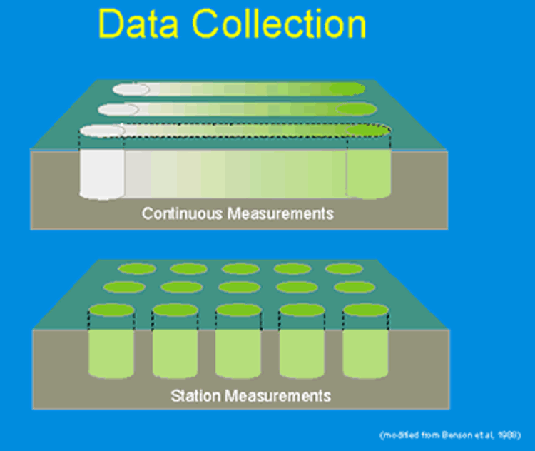
Figure 9. An example of continuous data collection versus station measurements for magnetic surveys (modified from Benson, et al., 1988).
Surveys are conducted in either a random pattern based on a statistical requirement or a grid. A grid is the most common layout for collecting magnetic data. Depending on the instrument, data are collected along traverse lines of the grid as either station measurements (proton precession magnetometers; bottom of Figure 9) or as nearly continuous measurements (proton Overhauser or optically pumped magnetometers; top of Figure 9). As noted in Table 2, data acquisition is faster for the Overhauser or optically pumped magnetometers (0.1-3 seconds) than for the older proton precession magnetometers (three to five seconds). The grid/traverse spacing is based on the estimated size of the target object. For smaller objects, a closer grid spacing is needed. The distance between traverses should be no further than the detectable range of the object. For example, if trying to locate a single drum, the spacing between traverse lines should be no more than six feet.
Data Display and Interpretation
Magnetic data consist of individual numeric values of total magnetic field intensity measurements or gradient measurements (Z value) along with location coordinates (X and Y values) for each measurement. Total field measurements are typically in the range of tens of thousands of gammas and are always positive since they are a direct value of the Earth's magnetic field plus or minus any values emanating from local fields. Gradient and corrected total field measurements are always smaller values. Because they consist of two total field measurements that are subtracted from each other, they provide only the value of the smaller local field emanating from the target object. These range from 0 (background) to several thousand gammas and can be positive or negative.
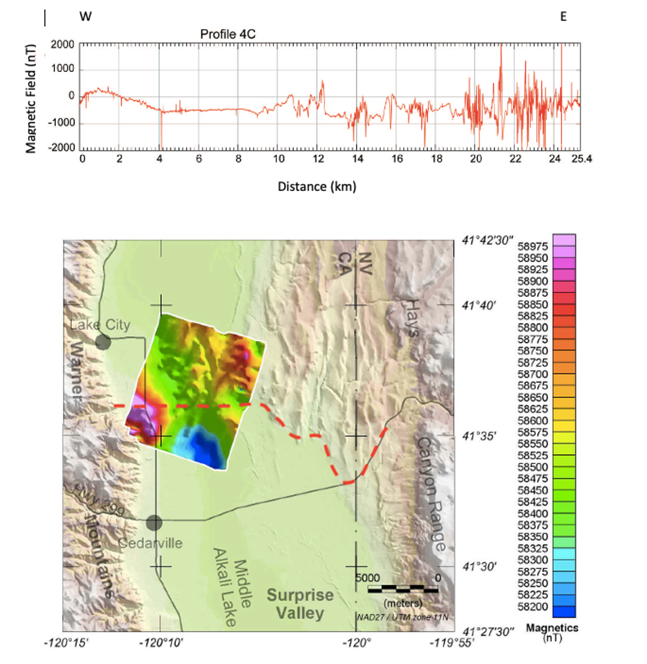
Figure 10. An example of magnetic data presented as a profile and a 2D map. The profile data were collected by a truck-towed system along the transect shown as a dashed red line. The 2D data were collected via an airborne platform (Ponce et al., 2009![]() ).
).
There are several ways to present magnetic data. Raw data can be listed in columns of X, Y, and Z data, but it can be difficult to visualize anomalous data. Data can also be presented as line graphs plotted for each line traversed with the magnetometer. Although this approach provides a graphic image of the data, it is difficult to relate each line to adjacent lines. Contour presentations provide a better perspective of the data. The contouring illustration can be modified by attaching a third dimension to the data based on the value of magnetic data to generate a net diagram, which provides a 3-dimensional perspective to a 2-dimensional data set. Figure 10 shows a profile and 2-dimensional presentation of magnetic data collected by airborne survey and by a truck-towed system. Combining multiple modes of data collection can provide additional lines of evidence for data interpretation. In this instance, the magnetic highs (in shades of red and pink) represent Tertiary and Quaternary volcanic rocks, and the magnetic lows (in shades of blue) are interpreted to be less magnetic Tertiary and Quaternary sedimentary rocks.
An experienced data analyst interprets magnetic data to ensure that an appropriate scale is used that will present all necessary details. Incorrect manipulation of contour scales can easily mask important anomalies. The interpreter must also remove interference from the data to avoid a false interpretation. Interpretation of the data should include discussions of data limitations and potential data gaps.
Figure 11 shows an example of a contour plot for one crushed drum aligned vertically, and the resulting magnetic field. In Figure 12, a group of five crushed drums yields a stronger magnetic signal.
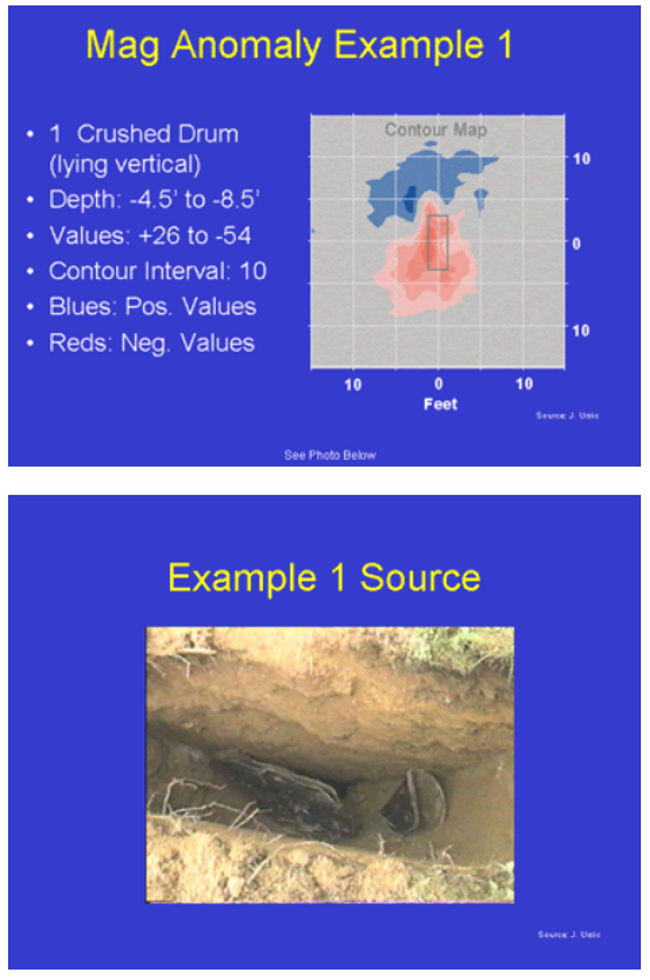
Figure 11. An example of a contour plot of a crushed buried drum (J. Ursic, EPA Region 5).
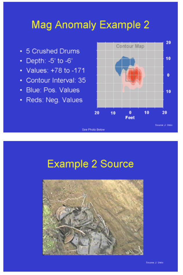
Figure 12. An example of a contour of the magnetic field detected from several crushed drums buried together (J. Ursic, EPA Region 5).
↩
Performance Specifications
The following performance specifications should be considered when collecting and interpreting magnetic data:
Interference
Three types of interferences can affect detection and sensing elements:
- External interferences: Electrical noise from AC power lines (proton precession magnetometers are also susceptible to DC voltage); transformers or other radiating transmitter sources; high magnetic gradients from underlying rocks/soil/minerals; nearby visible or hidden iron alloy objects (e.g., cars, railroad tracks, utility hole covers, fence lines, grates).
- Inherent interferences: Optically pumped magnetometers have a "dead zone," in which certain ambient magnetic field angles are undetected. The dead zone can be minimized by adjusting the sensor angle based on the latitude of the site and the incidence angle of the magnetic field lines.
- Solar interferences: Atmospheric effects are mainly a concern when a magnetometer is used in the total field mode9. Minimizing problems associated with this phenomenon can be resolved by using a gradiometer10 or obtaining total field measurements in conjunction with a properly set up base station.
Detection Limits
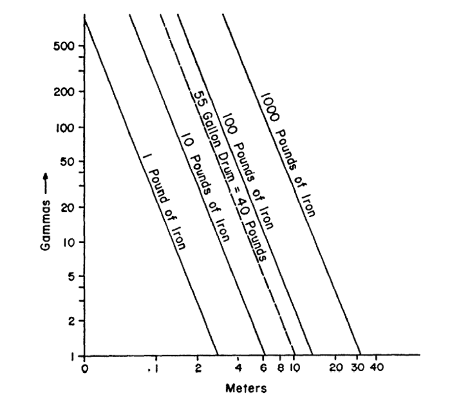
Figure 13. Estimated magnetometer response in gammas to objects of different mass at various depths (Benson, et al., 1984).
Detection limits for magnetometers vary according to the method. Older technologies such as fluxgate systems can have a detection limit of 10 gammas. Detection limits for proton precession tools and optically pumped systems are 0.1 or 0.2 gammas and about 0.01 gamma, respectively. Note that a detection limit is relevant only if the magnetic field of the object being evaluated is within range of the sensor so that the field can be distinguished from background. If a magnetic field of a buried ferromagnetic object does not extend beyond the ground surface, it will not be detectable no matter how small the detection limit. The detection limit unit (gammas) cannot be directly related to the depth or size of a target object. The response of the magnetometer varies by one over the distance (d) cubed (1/d3). Therefore, if the distance between the object and the magnetometer is doubled, the response will be decreased by a factor of eight (Benson, et al., 1984). For example, a 55-gallon drum that is buried approximately three meters deep can have a response of around 50 gammas. The same drum buried six meters deep may have an estimated response of around six gammas. Figure 13 provides estimates of magnetometer response in gammas for various object depths and mass.
Calibration
Generally, calibration is not needed for optically pumped magnetometers, if handled properly and not subjected to shock. Most magnetometers have a built-in self-test mechanism capable of evaluating their working condition. Although most proton precession magnetometers have onboard monitoring systems, they may also require a minor adjustment if the magnetometer's total field range was previously set for a field intensity significantly different (thousands of gammas) from the current background location. Such an adjustment is made through the instrument's onboard numeric keypad. The correct value can be checked by using a reference map showing the Earth's total magnetic field intensity and matching the general total field background value closest to your geographic location. Once an approximate value is entered for the geographic location, the instrument will be able to automatically fine-tune the value.
Quality Control
To ensure the quality of survey data:
- Monitor and evaluate solar activity – Daily information and forecasts of solar activity that may disrupt magnetic measures are available from NOAA. Knowledge of the solar activity allows the operator to determine the optimal time window to obtain total field measurements or when a gradiometer should be used.
- Collect background data – Select an area free of ferromagnetic materials to establish this point as background, then average several measurements at this location. Several times during the survey, the operator should return to the background point and resample. If the readings are similar, the instrument is performing properly.
- Use instrument monitoring systems – Some instrument manufacturers build in monitoring systems so that the operator can observe the functionality of the system during a survey.
- Determine operator-generated magnetic fields – Before each survey, the operator should keep the instrument stationary and obtain data while walking an equidistant circle around the instrument. If the data remain similar during this test, the operator is assured that nothing on the person was detectable by the sensor(s), which could bias the data.
Precision and Accuracy
Precision refers to the repeatability of the magnetic survey. This is important when changes to the Earth's magnetic field occur at the time of measurement or if subsequent surveys are compared. Errors introduced into the data by fluctuations in the Earth's magnetic field can be corrected by using a reference base station magnetometer. Subtracting the base station measurements from the survey data corrects for the temporal changes in the Earth's magnetic field. A base station is not required for gradiometers as this method eliminates time variations in the data (Benson, et al., 1984).
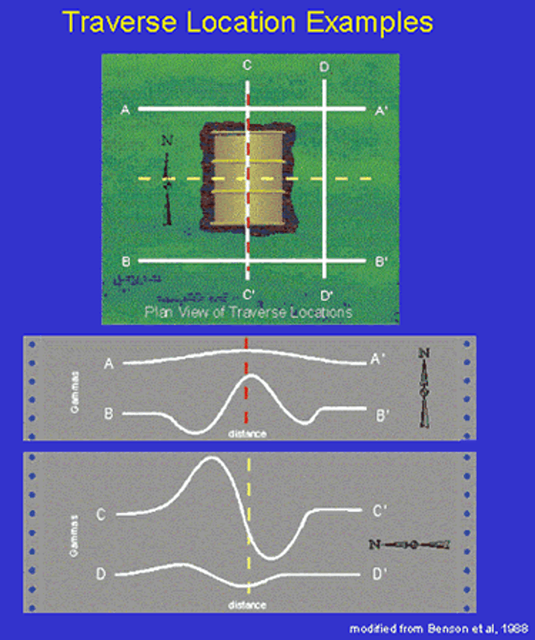
Figure 14. An example of how the location of the traverse affects the intensity of the magnetic field detected by the instrument (modified from Benson, et al., 1988).
Accuracy11 of data to locate the "true" location of an object depends on the experience of the person interpreting the data. Typically, an anomaly will have peaking positive and/or negative values due to the mass's composition and orientation, and how the sensor traversed over the target (Figure 14). An experienced data analyst can accurately pinpoint the center of an anomaly. However, a larger mass has a more extensive magnetic field that emanates from the main body and can be detected before reaching the target. Thus, the endpoints of a target may be accurate only within several feet. Smaller targets will not have large emanating fields, and thus, their extent can be established more accurately. Note that accuracy is mainly considered for defining lateral extents over a target. Depth estimates are difficult to determine unless details such as target shape, orientation, and mass are known and can be applied to a modeling program.
Depth of burial and geographic location also affect the accuracy of magnetic detection. The deeper the object, the longer the wavelength of its magnetic anomaly. Shallow buried objects have magnetic anomalies with shorter wavelengths. However, dispersed shallow objects which yield a broad magnetic anomaly can be mistaken for an object buried at depth (Benson, et al., 1984 and Grauch, et al., 2009![]() ). Additionally, the magnetic anomaly of a buried object will be offset from the actual object due to the angle of Earth's magnetic field at a particular latitude. Reduction to pole (RTP) corrections shift the observed location of the anomaly over the actual location of the object.
). Additionally, the magnetic anomaly of a buried object will be offset from the actual object due to the angle of Earth's magnetic field at a particular latitude. Reduction to pole (RTP) corrections shift the observed location of the anomaly over the actual location of the object.
Advantages
Advantages to using magnetometers include:
- They can detect ferromagnetic metals and their alloys.
- The magnetometer sensors, which collect ambient magnetic forces, are not subject to the same interference as ground penetrating radar.
- Most systems and support equipment (measuring tapes, GPS units, and flagging) can easily be transported in the trunk of a car or van.
- Systems are non-invasive, mobile, and self-contained. No external power or additional connections are needed.
- Definitions of lateral extents of mass are fairly accurate.
- Magnetic values often provide some indication of relative mass, i.e., large mass versus small mass.
- Most systems, except the conventional proton precession method, can obtain data at a walking pace (or faster), allowing an area of several acres to be surveyed in a day.
- Newer magnetometer systems have been designed with a direct input for GPS.
- Magnetometer systems are widely available for purchase or rental.
- Magnetics typically can "see through" certain interference that would limit other geophysical methods. For example, a steel tank at an unknown location beneath a paved parking lot (reinforced with wire mesh or rods) can be identified using a magnetometer. A magnetometer would be able to locate the tank since its magnetic field would be greater than that of the reinforcement material.
Limitations
Magnetometers have the following limitations to consider:
- Magnetometers are subject to magnetic fields from non-target ferromagnetic materials (e.g., fences, vehicles, buildings, ferromagnetic scrap and debris, natural soil minerals, above ground or underground utilities, and lightning) that may be on or near the survey area.
- When a single sensor is used, the resulting magnetic field intensity measurement is sensitive to atmospheric fluctuations in the Earth's magnetic field. Using gradiometers or base station measurements can correct for this phenomenon (Benson, et al., 1984
 ).
). - Depths may be difficult to estimate and vary based on the object's magnetic properties, geometry, orientation, condition, and its magnetic field.
- Skilled personnel are needed to configure the optimal data collection patterns and to analyze and interpret the results.
- Low batteries or low fluids (in proton precession systems) can cause errors.
- Temperatures greater than 149°F can damage the sensor in the Overhauser type magnetometer. The system operator must monitor temperature conditions to assure data quality.
- Magnetometers typically will not work inside buildings.
Cost
Cost estimates in Table 5 are based on estimates from magnetometer vendors. Rental and purchase costs do not include materials and tools needed to set up a grid, markers, or other locational devices. A geophysical field service contractor can provide an entire magnetometer survey from start to finish. Some contractors' base price options provide for data collection, but not a documented interpretation.
Table 5. Costs Estimates for Magnetometers
| Instrument Type | Equipment Purchase | Equipment Rental |
| Proton Precession (Conventional) | $6,000 | $30/day or $720/month |
| Proton Precession (Overhauser) | $8,100 | $120/day or $1,600/month |
| Optically Pumped | $14,500 | $80/day or $2,040/month |
Case Studies
Integrated Interpretation of Magnetic and ERT Data to Characterize a Landfill in the North-West of Cologne, Germany.
Ibraheem, I. et al., Pure Applied Geophysics, Vol. 178, pp. 2127-2148, May 2021
Electrical resistivity tomography and ground magnetic surveys were applied to characterize an old uncontrolled landfill in a former exploited sand and gravel quarry. These non-invasive geophysical tools helped portray the covering soil, the spatial limits of the landfill, and the depth of the waste body. They also successfully detected low resistivity zones at deeper depths than expected, which probably associated with migration pathways of the leachate plumes.
Assessment of Multiple Geophysical Techniques for the Characterization of Municipal Waste Deposit Sites
Gael, D, et al., Journal of Applied Geophysics, Vol. 145, pp. 74-83, October 2017.
This study tested the ability of geophysical methods, including magnetometers, to characterize a large technical landfill installed in a former sand quarry to delineate horizontal extent of the deposit site, estimating its thickness and characterizing the waste material composition (the moisture content in the present case).
![]() Geophysical Survey of the Los Angeles Landfill, Albuquerque NM
Geophysical Survey of the Los Angeles Landfill, Albuquerque NM
Crook, N., et al., RPT-2016-031, Rev. 0, September 2016.
A multi-method geophysical survey was performed at a closed landfill to determine the lateral extent and thickness of buried waste and the depth of cover material over the waste. A combined electromagnetic (EM) and magnetic (Mag) survey over the entire accessible landfill area, as well as seven lines of two-dimensional (2D) Electrical Resistivity Tomography (ERT), were completed.
Ground Magnetometric Surveys and Integrated Geophysical Methods for Solid Buried Waste Detection: A Case Study
Marchetti, M., et al., Annals of Geophysics, Vol. 45, No.3/4, June/August 2002.
The results of an investigation carried out in a tuff quarry in Italy are described. A preliminary magnetometric survey revealed the existence of anomalous zones, and excavation confirmed that the anomalies were generated by underground magnetic material. Over 160 steel drums were found. After their removal, a new magnetometric survey was performed. Based on the new map, a multifrequency induction survey, a geoelectrical profile and GPR measurements were taken to extend the characterization of the subsoil.
Testing of Airborne Vertical Magnetic Gradiometer System. Revision 1
Oakridge National Laboratory, Environmental Sciences Division, ESTCP Projects 200037 and 37, August 2005.
A prototype airborne vertical magnetic gradiometer system was tested and reported at three sites – Pueblo of Laguna, NM; Aberdeen Proving Ground, MD; and Badlands Bombing Range, SD.
Abandoned Underground Storage Tank Location Using Fluxgate Magnetic Surveying: A Case Study
Van Biersel, T. et al., Ground Water Monitoring and Remediation, Vol. 22, Issue 1, pp. 116-120, Winter 2002.
A fluxgate magnetometer survey, followed by confirmatory excavation, was conducted to locate a second onsite source of petroleum contamination.
Magnetometer Towed Array. Innovative Technology Summary Report
U.S. Department of Energy, Office of Environmental Management, Office of Science and Technology, DOE/EM-0502, pp. 25, September 1999.
This report provides an overview of the use of a magnetometer towed array to assess buried waste.
A Test Site for the Magnetic Detection of Buried Steel Drums
Marchetti M, et al., Annals of Geophysics, Vol. 41 No. 3, August 1998.
Magnetic techniques were performed to detect buried steel drums at a site in Central Italy.
↩References:
Benson, R., et al., 1984. Geophysical Techniques for Sensing Buried Waste and Waste Migration. EPA-600/7-84-064. 256 pp. June.
Benson, R, et al., 1988. Geophysical Techniques for Sensing Buried Wastes and Waste Migration. National Water Well Association Dublin, OH, 236 pp.
Ernstson, K., 2009. Groundwater Geophysics: A Tool For Hydrogeology, Chapter 9, pp. 275-282.
Grauch, V., et al., 2009. ![]() Geophysical Interpretations of the Southern Española Basin, New Mexico, That Contribute to Understanding Its Hydrogeologic Framework. U.S. Geological Survey Professional Paper 1761, 88pp.
Geophysical Interpretations of the Southern Española Basin, New Mexico, That Contribute to Understanding Its Hydrogeologic Framework. U.S. Geological Survey Professional Paper 1761, 88pp.
Indian Institute of Geomagnetism, 2018. Geomagnetic Field Measurements and Data. Accessed September 2021.
New Jersey Department of Environmental Protection, 2005. Field Sampling Procedures Manual. Chapter 8, August. 46 pp.
NASA. Measuring Earth's Magnetism. Accessed September 2021.
McGinnis, R., et al., 2011. ![]() Review of Geophysical Methods for Site Characterization of Nuclear Waste Disposal Sites. U.S. Nuclear Regulatory Commission Contract NRC-02-07-006. 29pp. October.
Review of Geophysical Methods for Site Characterization of Nuclear Waste Disposal Sites. U.S. Nuclear Regulatory Commission Contract NRC-02-07-006. 29pp. October.
Marine Magnetics Corporation, 2007. ![]() SeaSPY Technical Application Guide, rev1.4. 13 pp.
SeaSPY Technical Application Guide, rev1.4. 13 pp.
OpenEI, 2013. Ground Magnetics. Accessed September 2021.
Ponce, D, et al., 2009. ![]() Geophysical Studies in the Vicinity of the Warner Mountains and Surprise Valley, Northeast California, Northwest Nevada, and Southern Oregon. U.S. Geological Survey, Open-File Report 2009-1157, 25 pp., 2009.
Geophysical Studies in the Vicinity of the Warner Mountains and Surprise Valley, Northeast California, Northwest Nevada, and Southern Oregon. U.S. Geological Survey, Open-File Report 2009-1157, 25 pp., 2009.
SEG Wiki, 2018. Magnetic Methods. Accessed June 2022.
U.S. EPA, 1993. Subsurface Characterization and Monitoring Techniques. A Desk Reference, Volume 1. EPA/625/R-93/003a. 498 pp. May.
U.S. Geological Survey. Earth Core. Accessed September 2021.
Helpful Information
The condition of the metal object will affect the signal response detected by the magnetometer. If the metal object has been deformed, such as a crushed drum, the surface area is reduced yielding a weaker signal. Corrosion of metal objects has a similar effect (Benson et al., 1984). ↩
The condition of the metal object will affect the signal response detected by the magnetometer. If the metal object has been deformed, such as a crushed drum, the surface area is reduced yielding a weaker signal. Corrosion of metal objects has a similar effect (Benson et al., 1984). ↩
The surface area of the metal object is related to the strength of the signal detected by the magnetometer. An intact, uncorroded steel drum will have a stronger signal than a crushed or corroded steel drum as the surface area of the drum is reduced by both crushing and corrosion. ↩
The surface area of the metal object is related to the strength of the signal detected by the magnetometer. An intact, uncorroded steel drum will have a stronger signal than a crushed or corroded steel drum as the surface area of the drum is reduced by both crushing and corrosion. ↩
Other common names are proton, precession, and nuclear magnetometer. ↩
Other common names are proton, precession, and nuclear magnetometer. ↩
Other common names include cesium, potassium, cesium vapor, potassium vapor, alkali vapor, and optical magnetometer. ↩
Other common names include cesium, potassium, cesium vapor, potassium vapor, alkali vapor, and optical magnetometer. ↩
Nanotesla (nT) is a unit of measure of magnetism. It is equal to 1 gamma (γ) or 1 X 10.0E-05 gauss. A gauss is a unit of magnetic induction in centimeters per gram per second. ↩
Nanotesla (nT) is a unit of measure of magnetism. It is equal to 1 gamma (γ) or 1 X 10.0E-05 gauss. A gauss is a unit of magnetic induction in centimeters per gram per second. ↩
- Proton Precession Magnetometers: Conventional-Free Precession Type
During the 1950s, a more accurate method of measuring magnetic fields was developed to supersede the method used to locate submarines during World War II (fluxgate method). The conventional-free precession magnetometer measures the reaction of subatomic particles in a sample volume to external magnetic forces. A fluid containing a hydrogen-rich compound is used as a detector for sensing magnetic fields by manipulating and monitoring the reaction of protons in the fluid. The most common fluids used are hexane and decane since these fluids do not freeze as easily as water in colder climates.
To initiate the process, electrical coils are placed around a container of hydrogen-rich fluid and energized for a very short time. The random natural spin of the protons will align themselves to the induced direct current (DC). When the DC is removed from the coil, the protons will rotate back (precess) to their natural random state of spin (Figure 8). The rate at which this proton precession will occur depends on the ambient magnetic field near the container or sensor. Strong magnetic fields will force the protons to precess at a faster rate than weaker magnetic fields. The rate at which the protons precess back to normal is proportional to the magnetic field strength and thus provides a measurable value. It takes several seconds to cycle through the entire process before obtaining a measurement.
Proton precession data are usually collected in one of two ways over an area. One method is to sequentially number data each time a reading is recorded and tie each numeric value to a coordinate location. A more common method is to establish a grid system over the area to be surveyed and pre-program the magnetometer's internal data acquisition program to match the grid system. This method not only saves the operator time by automatically advancing to the next grid point, but it also reduces the chances for errors in the field. Data values and grid information typically are visible to the operator on the console of the control unit, which stores the data. Raw data for either method consist of time-stamped values, sequential numbering, X - Y positioning, sensor stability information, and sensor measurement data. Maintenance typically consists of replenishing the fluid and ensuring proper battery condition. Proton Precession Magnetometers: Conventional-Free Precession Type
During the 1950s, a more accurate method of measuring magnetic fields was developed to supersede the method used to locate submarines during World War II (fluxgate method). The conventional-free precession magnetometer measures the reaction of subatomic particles in a sample volume to external magnetic forces. A fluid containing a hydrogen-rich compound is used as a detector for sensing magnetic fields by manipulating and monitoring the reaction of protons in the fluid. The most common fluids used are hexane and decane since these fluids do not freeze as easily as water in colder climates.
To initiate the process, electrical coils are placed around a container of hydrogen-rich fluid and energized for a very short time. The random natural spin of the protons will align themselves to the induced direct current (DC). When the DC is removed from the coil, the protons will rotate back (precess) to their natural random state of spin (Figure 8). The rate at which this proton precession will occur depends on the ambient magnetic field near the container or sensor. Strong magnetic fields will force the protons to precess at a faster rate than weaker magnetic fields. The rate at which the protons precess back to normal is proportional to the magnetic field strength and thus provides a measurable value. It takes several seconds to cycle through the entire process before obtaining a measurement.
Proton precession data are usually collected in one of two ways over an area. One method is to sequentially number data each time a reading is recorded and tie each numeric value to a coordinate location. A more common method is to establish a grid system over the area to be surveyed and pre-program the magnetometer's internal data acquisition program to match the grid system. This method not only saves the operator time by automatically advancing to the next grid point, but it also reduces the chances for errors in the field. Data values and grid information typically are visible to the operator on the console of the control unit, which stores the data. Raw data for either method consist of time-stamped values, sequential numbering, X - Y positioning, sensor stability information, and sensor measurement data. Maintenance typically consists of replenishing the fluid and ensuring proper battery condition. ↩Proton Precession Magnetometers: Overhauser Type
An Overhauser proton precession magnetometer provides a slight technological improvement over the conventional-free precession magnetometer. The Overhauser type is basically the same as the conventional proton precession type except for differences in sensor fluid and type of current applied around the fluid. The proton-rich sensor fluid is spiked with free radicals to enhance the reactiveness of the protons to an electrical stimulus. Rather than applying high-power DC around the sensor, a low-power radio frequency magnetic field is applied for a very short time around the fluid. This type of system maximizes resolution and is more efficient since polarization and measurement of the protons occur almost simultaneously.
The sensors are sensitive to extreme heat and can be damaged if subjected to heat above 149°F. This type of tool should never be left in an unventilated vehicle on a hot day, and wrapping a wet, light-colored cloth around each sensor is recommended when working in direct sun light at a temperature above 100°F.
Data collection times are slightly faster than conventional-free precession methods and may allow the operator to collect data at a slow walking pace. Raw data, data storage, data collection techniques, and maintenance issues are similar to that of the conventional-free precession method discussed above. ↩Proton Precession Magnetometers: Overhauser Type
An Overhauser proton precession magnetometer provides a slight technological improvement over the conventional-free precession magnetometer. The Overhauser type is basically the same as the conventional proton precession type except for differences in sensor fluid and type of current applied around the fluid. The proton-rich sensor fluid is spiked with free radicals to enhance the reactiveness of the protons to an electrical stimulus. Rather than applying high-power DC around the sensor, a low-power radio frequency magnetic field is applied for a very short time around the fluid. This type of system maximizes resolution and is more efficient since polarization and measurement of the protons occur almost simultaneously.
The sensors are sensitive to extreme heat and can be damaged if subjected to heat above 149°F. This type of tool should never be left in an unventilated vehicle on a hot day, and wrapping a wet, light-colored cloth around each sensor is recommended when working in direct sun light at a temperature above 100°F.
Data collection times are slightly faster than conventional-free precession methods and may allow the operator to collect data at a slow walking pace. Raw data, data storage, data collection techniques, and maintenance issues are similar to that of the conventional-free precession method discussed above. ↩Optically Pumped Magnetometers (Cesium vapor or Potassium vapor)
A faster and even more accurate method of obtaining magnetometer measurements uses an ionizing light beam to manipulate one of several elements from a specific chemical group within a sample volume for the purpose of observing their reaction to external magnetic forces. By manipulating and monitoring the nuclei of any alkali metal (lithium, sodium, potassium, rubidium, cesium, or francium), the magnetic forces can be measured.
The optically pumped magnetometer exploits this phenomenon to measure magnetic fields (Figure 9). An alkali vapor, such as cesium or potassium, is sealed within a temperature-controlled vacuum chamber where ionizing light is emitted or "pumped" into the chamber through various optical filters. The ionizing light energizes the molecules in the sample volume and ejects electrons from the outermost orbit of individual electrons. Ambient magnetic fields near the vacuum chamber will tend to force the electrons back to their stable state. During this process the loss of energy due to the electrons dropping down to their stable state must be released and is given off as a spark of light. A photomultiplier tube (a device that measures light intensity) at the other end of the vacuum chamber measures the amount of light given off. Greater light intensity means that a strong magnetic field is quickly forcing electrons back to a normal state within the sample volume. Weaker magnetic fields will not cause the electrons to return to normal as rapidly, thus producing less light in the sample volume. The rate at which electrons revert to normal is proportional to the magnetic field strength and thus provides a measurable value.
Advantages to using optically pumped magnetometers are faster measuring cycles (as frequent as 0.1 second) and greater accuracy in measuring magnetic field strength. The tool must be handled with care in the field due to the fragility of the sensor. Optically pumped magnetometers have an inherent "dead zone" field of view in the sensor; however, properly orienting the sensors for a specific location or latitude (a relationship which determines angles of magnetic fields at a latitude) will reduce the "dead zone" effect and allow for an efficient measurement. Proper sensor angles are available from published charts, tables, or computer programs typically supplied by the magnetometer vendor.
Raw data consist of time-stamped values, sensor stability information, pre-programed grid line intervals (X-axis) with start and end markers to indicate all (Y-axis) data collected in each line, and averaged data posted at an operator-selected time interval. Newer systems also have inputs for global positioning systems (GPS). Maintenance typically consists of ensuring proper battery condition.
Optically pumped magnetometers are used most often for environmental field analysis since the technology is optimized for speed, sensitivity, and compatibility with GPS tools. ↩Optically Pumped Magnetometers (Cesium vapor or Potassium vapor)
A faster and even more accurate method of obtaining magnetometer measurements uses an ionizing light beam to manipulate one of several elements from a specific chemical group within a sample volume for the purpose of observing their reaction to external magnetic forces. By manipulating and monitoring the nuclei of any alkali metal (lithium, sodium, potassium, rubidium, cesium, or francium), the magnetic forces can be measured.
The optically pumped magnetometer exploits this phenomenon to measure magnetic fields (Figure 9). An alkali vapor, such as cesium or potassium, is sealed within a temperature-controlled vacuum chamber where ionizing light is emitted or "pumped" into the chamber through various optical filters. The ionizing light energizes the molecules in the sample volume and ejects electrons from the outermost orbit of individual electrons. Ambient magnetic fields near the vacuum chamber will tend to force the electrons back to their stable state. During this process the loss of energy due to the electrons dropping down to their stable state must be released and is given off as a spark of light. A photomultiplier tube (a device that measures light intensity) at the other end of the vacuum chamber measures the amount of light given off. Greater light intensity means that a strong magnetic field is quickly forcing electrons back to a normal state within the sample volume. Weaker magnetic fields will not cause the electrons to return to normal as rapidly, thus producing less light in the sample volume. The rate at which electrons revert to normal is proportional to the magnetic field strength and thus provides a measurable value.
Advantages to using optically pumped magnetometers are faster measuring cycles (as frequent as 0.1 second) and greater accuracy in measuring magnetic field strength. The tool must be handled with care in the field due to the fragility of the sensor. Optically pumped magnetometers have an inherent "dead zone" field of view in the sensor; however, properly orienting the sensors for a specific location or latitude (a relationship which determines angles of magnetic fields at a latitude) will reduce the "dead zone" effect and allow for an efficient measurement. Proper sensor angles are available from published charts, tables, or computer programs typically supplied by the magnetometer vendor.
Raw data consist of time-stamped values, sensor stability information, pre-programed grid line intervals (X-axis) with start and end markers to indicate all (Y-axis) data collected in each line, and averaged data posted at an operator-selected time interval. Newer systems also have inputs for global positioning systems (GPS). Maintenance typically consists of ensuring proper battery condition.
Optically pumped magnetometers are used most often for environmental field analysis since the technology is optimized for speed, sensitivity, and compatibility with GPS tools. ↩-
In total field mode, the magnetometer has only one sensor measuring the strength of the local magnetic field. The magnetic field that is measured is comprised of the Earth's magnetic field, atmospheric disturbances, and the anomaly. This mode is susceptible to atmospheric disturbances that could mask small anomalies. See Figure 8 and Table 2. ↩
-
In total field mode, the magnetometer has only one sensor measuring the strength of the local magnetic field. The magnetic field that is measured is comprised of the Earth's magnetic field, atmospheric disturbances and the anomaly. This mode is susceptible to atmospheric disturbances, that could mask small anomalies. See Figure 8 and Table 2. ↩
A gradiometer consists of two magnetometers with their sensors separated either vertically or horizontally. The field gradient caused by the magnetic anomaly is calculated by the difference between the two sensed magnetic fields. This method eliminates inferences caused by atmospheric disturbances that could mask small anomalies. See Table 2. ↩
A gradiometer consists of two magnetometers with their sensors separated either vertically or horizontally. The field gradient caused by the magnetic anomaly is calculated by the difference between the two sensed magnetic fields. This method eliminates inferences caused by atmospheric disturbances that could mask small anomalies. See Table 2. ↩
Accuracy is a measure of how close the result of an analysis comes to the "true" locational estimation of an anomaly. ↩
Accuracy is a measure of how close the result of an analysis comes to the "true" locational estimation of an anomaly. ↩